Machine Learning › Machine Learning Fundamentals › Day 145
Day 145: Overfitting and Underfitting
After this lesson you will treat overfitting and underfitting as two different quantities rather than two ends of one dial, because you will have measured both directly. You will fit 200 models to 200 independent training sets and separate bias from variance by brute force, then watch the three parts -- bias squared, variance and irreducible noise -- add up to the error that was actually observed, to within one percent at every capacity. You will see a degree-1 model score BETTER on data it has never seen than on its own training set, and understand that the negative gap is the signature of underfitting rather than a bug in the split. You will watch test error fall to 5.4911 at degree 4 and climb to 226,667 at degree 24 while training error falls the whole way. You will rescue that same degree-24 model with a ridge penalty, improving its test error by a factor of 39,588 while deliberately making its training error worse. You will measure the sentence this whole lesson exists for: more data took an overfit model from 215,413 down to the 4.0 noise floor and an underfit one from 8.5023 to 8.2393. And you will find, by accident, the interpolation threshold -- the point where 25 features meet 25 rows and everything falls apart.
Hands-on lab for this lesson
Lab files on GitHub: https://github.com/ai-roadmap-365/ai-roadmap-365.github.io/tree/main/labs/sections/machine-learning/day-145-overfitting-and-underfitting
- Get the hands-on files. Clone the labs repository once (you can reuse this clone for every lesson). This works on macOS, Linux, and Windows (PowerShell or WSL):
git clone https://github.com/ai-roadmap-365/ai-roadmap-365.github.io.git cd ai-roadmap-365.github.io - Open this lesson's lab. Move into the directory for this specific day. Every lab lives at the same predictable path — section / subsection / week / day:
cd labs/sections/machine-learning/day-145-overfitting-and-underfitting - Read the lab guide. Open `README.md` in that directory. It lists the exact commands, what each does, the expected output, and how to check your work — read it before running anything.
- Run it and check your work. Follow the README's "How to run" section: run the example first to see the finished result, then complete the numbered exercises in `starter/`, then run the tests. The tests pass (exit 0) only when your work is correct.
bash tests/run_tests.sh # or the test command named in the lab README
You can also open the lab as a local page (works offline, shows the file tree and expected output).
Learning objectives
By the end of this lesson you will be able to:
- Separate overfitting from underfitting as distinct quantities -- variance and bias -- rather than as two ends of one capacity dial
- Measure bias and variance directly by fitting many models to many independent training sets
- Verify that bias squared plus variance plus noise equals the error actually observed
- Diagnose which failure a model has from the sign of its generalisation gap, using a single fit
- Recognise a negative gap as the signature of underfitting rather than as a broken split
- Explain why a strictly larger model class can carry more bias as well as more variance
- Predict which interventions help each failure, and name the expensive mistake each diagnosis rules out
- Tune a regularisation penalty and explain why the training error rising is the mechanism rather than a side effect
- Estimate the irreducible noise floor and use it to decide when to stop spending
- Treat training time as a capacity dial, and explain why early stopping needs patience rather than a first-increase rule
- Identify the interpolation threshold where the number of features meets the number of rows
- Distinguish overfitting from Day 144's selection bias, and say why regularising cannot fix the latter
Prerequisites
- Day 141 -- a training score is arithmetic rather than evidence; a 1-NN scores 1.000 on coin flips
- Day 143 -- the workflow, and that anything fitted is fitted on training rows only
- Day 144 -- three sets, the generalisation gap, and selection bias, which this day is repeatedly careful to distinguish from overfitting
- Days 117-118 -- the sampling distribution, which is what the variance term is measuring
- Day 111 -- gradient descent and the learning-rate regimes, which is what the early-stopping measurement is running
- Comfort with NumPy arrays and reading a pytest failure, and a working python3 3.11 or newer on your PATH; the lab builds its own virtual environment and needs no GPU
Why this matters
Here are two models fitted to the same twenty-five points.
   deg    train MSE        test MSE             gap
     1      11.3217          9.8274         -1.4942
    24       1.0321     226667.4689     226666.4368
The second one fits its training data eleven times better. On data it has not seen, it is worse by a factor of twenty-three thousand.
That much is the familiar story, and if it were the whole story this lesson would be one paragraph long: do not use too much capacity. But look at the first row again, at the column on the right.
The gap is negative. The degree-1 model scores better on data it has never seen than on the data it was fitted to — 9.83 against 11.32. That is not a rounding artefact and it is not luck. It is the signature of the other failure, the one nobody watches for, and it happens for a reason worth understanding: a model too rigid to chase the noise in its training set has no noise-chasing to be flattered by, so its training score carries none of the usual optimism.
Two failures, then, and they are not two ends of one dial that you tune by feel. They are two different quantities, they respond to completely different interventions, and today’s lab measures both of them directly:
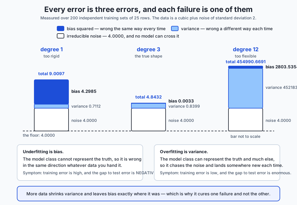
   deg     bias^2       variance      noise      predicted     observed
     1      4.2985         0.7112     4.0000         9.0097         9.0295
     3      0.0033         0.8399     4.0000         4.8432         4.8431
    12   2803.5354    452183.1336     4.0000    454990.6691    455027.8625
Read the first two columns across the rows and the whole subject is there. Underfitting is bias: at degree 1 the model is wrong by 4.30 in a way that no amount of new data will change, because a straight line cannot be a cubic no matter how many points you show it. Overfitting is variance: at degree 12 the bias is a rounding error next to 452,183 of scatter, because the model lands somewhere completely different for every training set it sees.
And the last two columns are the reason this is a lesson rather than an analogy. The three parts add up to the error that was actually observed, at every capacity, to within one percent. This is not a metaphor about archery targets. It is an identity, and today’s lab checks it.
The practical payoff arrives in the third measurement:
      n    degree 1     degree 4        degree 24
     15      8.5023      4.9218      215413.2388
   2000      8.2393      3.9880           4.0055
A hundred and thirty times more data took the overfit model from 215,413 to 4.0055 — which is the irreducible noise floor, exactly. It took the underfit model from 8.50 to 8.24.
More data cures one of these failures completely and the other one not at all. If you cannot tell which you have, you cannot tell whether the most expensive thing you could do next would help.
The idea in plain language
Two ways to be a bad witness.
The first witness is rigid. Whatever happened, they will tell you the story they always tell: it was a man in a dark coat, it happened quickly, it was probably about money. Ask them about a different crime and you get the same account. They are consistent, reliable and reproducible, and they are consistently wrong in the same direction — because their account was decided before they arrived. That is bias, and a witness like that does not improve when you show them more evidence. They have already decided what evidence looks like.
The second witness is suggestible. They remember everything, including things that did not happen. Ask them twice and you get two different stories, both vivid, both full of detail, neither reliable. They are not wrong in a direction; they are wrong in every direction at once, and which way depends entirely on what happened to be in front of them. That is variance, and this witness does improve when you show them more evidence — enough of it, and the invented detail averages out.
And then there is the third thing, which is neither witness’s fault: some of what happened genuinely was not visible from where anybody stood. That is irreducible noise. No witness, however good, gets past it.
The reason this analogy earns its place is the diagnostic it suggests. You cannot tell the two witnesses apart from a single interview — both will sound confident. You tell them apart by interviewing them repeatedly. The rigid one says the same wrong thing every time; the suggestible one says something new every time.
That is exactly what today’s lab does. It fits two hundred models to two hundred independently drawn training sets, and asks two questions: how far is the average prediction from the truth, and how far do the individual predictions scatter from their own average? The first is bias. The second is variance. Neither is visible from one fit, which is precisely why both are so easy to misdiagnose.
Historical background
The decomposition is older than the vocabulary around it.
In statistics, the trade-off between a biased estimator with low variance and an unbiased one with high variance was well established by the middle of the twentieth century. Stein’s paradox in 1956 — that a deliberately biased estimator can beat the obvious unbiased one on mean squared error in three or more dimensions — is the same idea arriving in a form that startled people, and it is still startling.
Ridge regression, which today’s lab uses to rescue a hopeless model, was published by Hoerl and Kennard in 1970 for exactly this reason. Their argument was not about machine learning; it was that when predictors are correlated the ordinary least-squares estimate has enormous variance, and that accepting a little bias buys a great deal of it back. That is the whole of regularisation in one sentence, fifty-five years ago.
The specific phrase “bias-variance dilemma” entered neural-network research with Geman, Bienenstock and Doursat in 1992, whose paper argued that the dilemma was the central obstacle for the field. Vapnik and Chervonenkis had by then supplied the other half of the picture from the 1970s onward: VC dimension gives a capacity measure and a bound relating training error to test error, and structural risk minimisation is the formal version of choosing capacity rather than maximising it.
Early stopping — today’s fifth measurement — has an equally respectable history and a slightly embarrassing origin: it was folklore among practitioners for years before anyone showed why it worked. The modern understanding is that stopping gradient descent early is, for linear models, closely related to an explicit penalty, which is why the two produce such similar curves.
One honest note about the modern picture. The clean U-shaped curve this lesson measures is real, it is what happens in the regime this lab constructs, and it is the right mental model for the models you will meet for the next several courses. It is also not the whole story for very large models: “double descent”, described in work from around 2019, observes test error falling again past the point where a model can interpolate its training data exactly. Today’s lab brushes against that boundary and the lesson says where, but the U-curve is what to internalise first, because it is what governs everything you will actually fit by hand.
What it is — and what it is not
Overfitting is not “the model is too complicated”. It is the model having enough freedom to fit the noise in this particular training set, so that what it learned includes things that will not be true next time. A complicated model on enough data does not overfit; a simple model on three points can.
Underfitting is not “the model is too simple” either. It is the model class being unable to represent the truth, so that the error survives however good the fit is. The distinction matters because it tells you the fix: no amount of optimisation, tuning or data will help a straight line approximate a cubic.
Here is the precise version. The expected squared error at a point decomposes into exactly three terms:
error = bias squared + variance + irreducible noise- Bias is how far the average prediction — averaged over training sets — sits from the truth. An error the model class makes every time.
- Variance is how much individual predictions scatter around that average. An error that changes with the training set.
- Noise is the part of the target that nothing could predict.
Today’s lab measures all three by brute force — two hundred training sets, two hundred fitted models, one fixed grid of query points — and then checks the sum against the error actually observed:
| degree | bias² | variance | noise | predicted | observed |
|---|---|---|---|---|---|
| 1 | 4.2985 | 0.7112 | 4.0000 | 9.0097 | 9.0295 |
| 3 | 0.0033 | 0.8399 | 4.0000 | 4.8432 | 4.8431 |
| 6 | 0.0108 | 4.3195 | 4.0000 | 8.3303 | 8.4147 |
| 12 | 2803.5354 | 452183.1336 | 4.0000 | 454990.6691 | 455027.8625 |
The worst disagreement across seven capacities is one percent, and that one percent is the Monte Carlo error in the observed column rather than a failure of the identity. At degree 3 the two agree to four decimal places.
Now the things this is not.
More capacity does not always mean less bias. This is worth dwelling on because the mental model of “one dial from rigid to flexible” predicts otherwise. Degree 2 is a strictly larger model class than degree 1 — every straight line is also a parabola with a zero quadratic term — and yet:
     1      4.2985         0.7112
     2      4.3342         1.4204
Degree 2 has more bias than degree 1, and double the variance. The
true function here is odd (0.5x³ − 2x + 1 has no even term worth
having), so the quadratic term can buy nothing and still costs. It is
worse on both counts than the smaller class it contains.
And a training score is not a diagnosis. Both failures can produce any training score you like. What distinguishes them is the gap, and the sign of the gap is the tell:
| capacity | gap | what it means |
|---|---|---|
| degree 1 | −1.4942 | underfitting — nothing was memorised, so nothing flatters the training score |
| degree 4 | +2.9948 | about right — a small honest gap |
| degree 24 | +226666.4368 | overfitting — the gap is the error |
Why it was created and what problems it solves
The decomposition exists because “the model is not good enough” is not an actionable statement, and the three terms turn it into three different actionable ones.
If your error is bias, the fixes are: a larger model class, better features, or a different model family. What will not help is more data, more training, or more tuning.
If your error is variance, the fixes are: more data, regularisation, a smaller model class, ensembling, or stopping earlier. What will not help is a more expressive model.
If your error is noise, nothing helps, and the useful action is to stop spending money. Today’s data has a noise standard deviation of 2.0, so the floor is exactly 4.0, and two of the three models reach it:
2000 8.2393 3.9880 4.0055At two thousand rows, the degree-4 model scores 3.9880 and the degree-24 model 4.0055. Both are at the floor, approaching it from opposite sides, and no further work on either is worth anything. Knowing that number — or estimating it — is what turns “we could probably squeeze out another point” into a decision.
Regularisation solves variance without giving up the model class, and the measurement is startling:
| alpha | train MSE | test MSE |
|---|---|---|
| 0.0 | 1.0321 | 226667.4689 |
| 0.001 | 1.5741 | 128.3127 |
| 1.0 | 2.7461 | 5.7257 |
| 10.0 | 3.9689 | 6.1559 |
| 100.0 | 6.2800 | 6.7840 |
The same degree-24 model, on the same twenty-five rows. A ridge penalty of 1.0 improves the test error by a factor of 39,588, and the best-regularised degree-24 model (5.7257) lands within half a point of the best unregularised degree-4 model (5.4911) — the same destination, reached from a completely different direction.
Two things in that table are worth naming. The training column rises monotonically with the penalty, always, because the penalty can only make the training fit worse: that is the trade, stated in numbers. And the test column is U-shaped in the penalty too — 100.0 is worse than 10.0 is worse than 1.0 — because too much regularisation is just underfitting by another route.
How it works
Measuring bias and variance directly
The identity is usually presented and then left alone, because measuring its terms requires something you never have in practice: many independent training sets and knowledge of the true function. In a lab you have both.
predictions = np.empty((datasets, grid))
for i in range(datasets):
    X_train, y_train = make_data(n_train, 10_000 + i)
    model = polynomial_model(degree).fit(X_train, y_train)
    predictions[i] = model.predict(query)

mean_prediction = predictions.mean(axis=0)
bias_squared = float(np.mean((mean_prediction - truth) ** 2))
variance = float(np.mean(predictions.var(axis=0)))
Two hundred models, each fitted to its own training set, all predicting the same fixed grid. Bias is how far the column mean sits from the truth; variance is how much the column scatters. Neither is computable from one fit, which is exactly why both are so easy to misdiagnose in practice — and why the gap, which is computable from one fit, is the diagnostic worth carrying.
The capacity curve, and why the axis has to be logarithmic
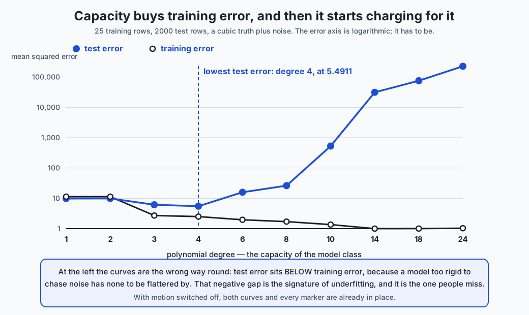
   deg    train MSE        test MSE             gap
     1      11.3217          9.8274         -1.4942
     2      11.3173          9.8801         -1.4372
     3       2.7076          6.1230          3.4154
     4       2.4964          5.4911          2.9948
     6       1.9569         15.8217         13.8648
     8       1.7010         26.1708         24.4697
    10       1.3570        528.4798        527.1227
    14       0.9685      31307.2782      31306.3097
    18       1.0037      75539.3618      75538.3581
    24       1.0321     226667.4689     226666.4368
Training error falls at every step through degree 14. Test error falls to 5.4911 at degree 4 and then rises by more than four orders of magnitude. That is why the diagram plots error on a log axis: on a linear one, every point except the last would be indistinguishable from zero.
One honest note on that training column. It falls monotonically through degree 14 and then wobbles by 0.0636 — 0.9685, then 1.0037, then 1.0321. That wobble is numerical rather than statistical. The training set has twenty-five rows, and degree 24 supplies exactly twenty-five polynomial features, so the fit is solving a square, catastrophically ill-conditioned system. Nothing about learning theory is involved; it is floating-point arithmetic running out of road. The lab asserts the monotonicity through degree 14 and asserts that it does not hold overall, rather than pretending the curve is clean.
That same coincidence — twenty-five features for twenty-five rows — explains something else the lab measures.
The interpolation threshold, found by accident
The third experiment sweeps training-set size at three fixed capacities, and the degree-24 column does something the story does not predict:
      n    degree 1     degree 4        degree 24
     15      8.5023      4.9218      215413.2388
     25      8.8620      6.1904    64631547.2994
     50      8.2457      4.2661        6070.3302
    100      8.3583      4.2934           5.3571
    400      8.3007      3.9958           4.3139
   2000      8.2393      3.9880           4.0055
More data makes it worse before it makes it better. From fifteen rows to twenty-five, the test error rises by a factor of three hundred, to sixty-four million.
That is not a bug, and the cause is exactly the coincidence above. Degree
24 supplies twenty-five features. At n = 25 the system is square: there
is exactly one solution, it interpolates every training point, and it is
under no constraint whatsoever about what happens between them. At
n = 15 there are more features than rows, the system is
under-determined, and least squares returns the minimum-norm solution
— which is, quietly, a form of regularisation, and behaves better.
The worst place to be is exactly at the threshold. That is the shape “double descent” describes, and today’s lab arrives at its left-hand edge without going looking for it. The lesson names it, measures the peak, and leaves the rest to the literature.
More data, and what it cannot buy
Set the threshold aside and read the three columns as a whole.
The degree-1 column spans 0.6227 across a hundred-and-thirty-fold increase in data, and ends within 0.3 of where it started. The degree-24 column falls by more than seven orders of magnitude and lands on the noise floor.
That is the practical content of the whole lesson. More data is a cure for variance and does nothing whatever for bias. If you are about to spend three months labelling, the question that decides whether it is worth it is which of these two you have — and the gap tells you, from a single fit, for free.
Training time is a capacity dial too
The last measurement changes only one thing: how long the fit is allowed to run. Same data, same model, same everything.
  training error falls every epoch  : True
  training error, first to last     : 7.3906 -> 2.4744
  best test error                   : 5.4555 at epoch 14
  test error at epoch 600           : 5.8978
  generalisation gap, epoch 1       : 0.6771
  generalisation gap, epoch 600     : 3.4234
Training error decreases at every one of six hundred epochs. The model gets monotonically better at the data in front of it, forever. Test error bottoms at epoch 14 and is worse at epoch 600, and the gap grows by a factor of five.
So capacity is not only a property of the model class. Gradient descent increases effective capacity as it runs, and stopping is a way of choosing less of it — which is why early stopping and an explicit penalty produce such similar curves.
One honest observation, because it changes the advice. The test curve is not a clean U. After its minimum it rises to 7.1435 around epoch 84, then partly recovers to 5.8978 by epoch 600 — without ever again beating the 5.4555 it reached at epoch 14. Five hundred and ninety-nine of the six hundred epochs are worse than the best one.
On this run, every patience setting from 5 to 50 recovers epoch 14 exactly, and so does a naive stop-at-first-increase. But that is luck on this run rather than a property of the rule: a curve that wanders like this one will, on another seed, dip below a local rise and defeat a naive stop. That wandering is the entire reason real implementations use patience and restore the best weights rather than the last ones.
An everyday analogy
Learning to cook from a single dinner party.
The underfitter takes one lesson from the evening: add more salt. They apply it to every dish for the rest of their life — soups, cakes, salads. It is a real lesson, drawn from real evidence, and it is approximately right on average. It will never get better, because they were never going to notice anything else. Cook them a thousand more dinners and they will still say “add more salt”, with the same confidence and the same partial success. More evidence changes nothing, because their capacity to absorb it was the constraint.
The overfitter takes away everything. The chicken was good, and there were seventeen guests, and it was raining, and the oven light was flickering, so now they cook chicken for exactly seventeen people in wet weather with a faulty bulb. Every one of those was genuinely present in the evidence. Only one of them mattered, and nothing in one dinner party distinguishes them.
Now the part that makes the analogy do work. Send the overfitter to forty dinner parties. The rain will have stopped for some, the guest count will vary, the bulb will be fixed — and the incidental details average out, leaving the chicken. Send the underfitter to forty dinner parties and they will tell you to add more salt.
That is the measurement, in a sentence. Forty dinners is 215,413 falling to 4.0055, and it is 8.5023 staying at 8.2393.
And the irreducible noise? Some of what made the evening good was the company, and no amount of technique will reproduce it. There is a floor, and today’s is exactly 4.0000.
Examples in practice
Diagnosing from the gap, which is all you usually have
In a real project you have one training set and no true function, so bias and variance are not directly measurable. What you always have is the gap, and it is enough to act on:
| What you see | Diagnosis | What to do |
|---|---|---|
| Training error high, gap near zero or negative | Underfitting | More capacity, better features. Not more data |
| Training error low, gap large | Overfitting | More data, regularisation, less capacity, stop earlier |
| Training error low, gap small, still not good enough | Near the noise floor | Estimate the floor before spending anything |
The negative-gap row is the one people miss, and today’s degree-1 model shows it plainly at −1.4942. An engineer who sees test error below training error usually assumes a bug in the split. Sometimes it is. Often it is a model with no capacity to overfit, and the fix is the opposite of the one they are about to apply.
Regularisation in the models you will actually use
The mechanism generalises well beyond ridge regression, and it is worth recognising the same idea in its various costumes:
- L2 (ridge) shrinks coefficients toward zero — today’s measurement, a factor of 39,588.
- L1 (lasso) drives some coefficients to zero, so it selects features as well as shrinking.
- Dropout, in neural networks, removes random units during training so no single unit can be relied on.
- Max depth and min samples per leaf, in trees, cap how finely the model may carve the space.
- Early stopping, today’s fifth measurement, limits how much of the available capacity gradient descent actually reaches.
Every one of these is variance reduction bought with bias. In each case the training error gets worse and that is the point, which is why a team that tunes for training error will reliably tune all of them off.
The learning curve as a spending decision
Plot training and test error against training-set size, and the shape tells you what your money buys.
If the two curves have converged and sit high, you are bias-limited: more data will change nothing, and the honest recommendation is a different model or better features. If a wide gap is still closing, you are variance-limited: more data will help, and the curve tells you roughly how much.
Today’s data sweep is that diagnosis run in advance. At n = 400 the
degree-24 model is at 4.3139 against a floor of 4.0, so the remaining
sixteen hundred rows buy 0.3 — and if labelling costs anything at all,
that is a decision, not a shrug.
The measurement that changes what people believe
The one to quote in a design review is the pair of columns from the data sweep, side by side: 215,413 to 4.0055, and 8.5023 to 8.2393. Same increase in data, same test set, same everything except which failure the model has. It is the fastest way to establish that “get more data” is a treatment rather than a tonic.
Implications: security, privacy, performance, scalability, and cost
The cost this lesson governs is the largest one in most projects: the decision to buy more labelled data. That decision is worth exactly what today’s data sweep measures, and it is worth nothing at all if the error is bias. Running a learning curve costs a few fits and answers the question before the money is spent.
Overfitting is a privacy problem as well as an accuracy problem. A model with high variance has, in a literal sense, stored particulars of its training rows — which is precisely what membership-inference attacks exploit. The regularisation that reduces variance also reduces memorisation, so the same intervention improves both. It is one of the few places where the privacy fix and the accuracy fix are the same fix.
Underfitting has a fairness dimension that is easy to miss. A model with too little capacity fits the majority pattern and is wrong in a consistent direction on everything else — and “consistently wrong in one direction on a subgroup” is what a fairness audit finds. Adding capacity can genuinely be the fairer choice, which cuts against the instinct that simpler models are safer.
Regularisation is nearly free; more data is not. A penalty is one hyper-parameter and a handful of extra fits to tune. The measurement here was a factor of 39,588 for one number. Before commissioning a labelling programme, tune the penalty.
And the noise floor is the number that stops a project spending forever. Estimating it is not always easy — repeated measurements of the same item, or agreement between human labellers, are the usual routes — but an estimate is enormously more useful than none. Today’s floor is 4.0000 and the best model is at 3.9880. There is nothing left to buy, and knowing that is worth more than another month of tuning.
Alternatives: free, open source, and commercial
Ridge and Lasso in scikit-learn — used here
When to choose them: as the first thing you try when a model overfits.
Free, BSD-3-Clause, no paid tier. Ridge for shrinkage, Lasso when you
also want feature selection, ElasticNet for both.
How to use them: one parameter, alpha, and it is worth tuning
properly. RidgeCV and LassoCV do the cross-validated search for you.
Today’s sweep found the best alpha at 1.0, with 10.0 and 100.0 both worse
— the penalty has its own U-curve.
Watch for: the scale of the features. A penalty on coefficients is a penalty in whatever units the features happen to be in, so an unscaled feature is effectively unpenalised. Today’s pipeline scales first, and that is not decoration.
validation_curve and learning_curve — used here in spirit
scikit-learn ships both as helpers. validation_curve sweeps one
hyper-parameter and returns train and validation scores;
learning_curve sweeps training-set size and returns the same. Today’s
lab computes both by hand so the mechanism is visible, but in a real
project the library versions are what you should reach for — they handle
the cross-validation correctly, which is the part that is easy to get
wrong.
Ensembles — described from documentation, not measured here
Bagging reduces variance by averaging models fitted to bootstrap resamples: many high-variance models, averaged, give a lower-variance one. Random forests are bagging plus feature subsampling. Boosting works from the other end, fitting many high-bias models in sequence, each correcting the last.
The framing worth carrying is that bagging attacks the variance term and boosting attacks the bias term, which is why they behave so differently when you tune them. No output from either is reproduced in this lesson; the description comes from scikit-learn’s documentation.
Automated hyper-parameter tuning services — not used here
Managed services search hyper-parameter space for you, including the regularisation strength this lesson tunes by hand.
When to choose one: when the search space is large and the fits are expensive enough that a smarter search than a grid pays for itself.
When not to: when you have not yet established which failure you have. A tuner will happily spend a large budget optimising the regularisation of a model whose problem is bias.
Free versus paid: the open-source libraries in this space are free; the managed services are paid and generally metered on compute. No price is quoted here, because these change by region and by month and an unchecked figure is worse than none.
Comparison with related concepts
| Concept | What it is | How it relates |
|---|---|---|
| The generalisation gap | test error minus training error | The diagnostic available from one fit; its sign distinguishes the two failures |
| Regularisation | a penalty on model complexity | Buys variance reduction with bias; measured here at a factor of 39,588 |
| Early stopping | limiting training iterations | The same trade, applied to effective rather than declared capacity |
| Model capacity | how much the model class can represent | Not a single dial: degree 2 has more bias AND more variance than degree 1 |
| VC dimension | a formal capacity measure | The theory that makes “capacity” precise rather than intuitive |
| Irreducible error | the part nothing can predict | Today’s floor of 4.0000; the number that stops a project spending |
| Double descent | test error falling again past interpolation | Where today’s degree-24 column peaks at n=25, and where the U-curve stops being the whole story |
| Selection bias | optimism from choosing on a set | Day 144’s subject; distinct from overfitting, and often confused with it |
The last row deserves a note, because the confusion is common and consequential. Overfitting is a model fitting its training data too closely. Selection bias is you fitting your choice of model to a validation set. They have different causes, different fixes, and different measurements — Day 144’s 0.5720-against-0.4992 has nothing to do with model capacity, and today’s 226,667 has nothing to do with how many models were compared. A team that regularises harder to fix a selection problem will make no progress at all.
When to use it — and when not to
Diagnose before you treat, and the gap is the diagnosis. Fit something, look at training error and the gap, and let the table above choose your next move. This costs one fit and routinely saves months.
Suspect underfitting when the gap is small or negative. A negative gap is not a bug report; it is a model with no capacity to overfit. The correct response is more capacity, and it is the opposite of what most people reach for.
Regularise before you buy data. One hyper-parameter, a handful of fits, and today’s measured factor of 39,588. Reversing that order is how projects spend a quarter’s budget on labels they did not need.
Estimate the noise floor early, even roughly. Repeated measurements or inter-annotator agreement will do. Without it there is no principled point at which to stop, and teams stop when they run out of enthusiasm instead.
Do not tune for training error, ever. Every variance-reducing intervention makes training error worse. That is what they are for, so a process that optimises training error will systematically switch all of them off.
And do not reach for capacity as a first move. Today’s degree-2 model is a strictly larger class than degree-1 and is worse on both bias and variance. Capacity is not a dial that runs from “worse” to “better”; it is a choice about which functions you are willing to consider, and a larger set is not automatically a better one.
The AI thread
Modern deep learning appears, at first glance, to refute everything above. Models with billions of parameters — vastly more than their training examples — are trained to near-zero training loss and generalise superbly. On the U-curve in this lesson, that should be catastrophic.
Three things reconcile it, and each is a version of something measured here.
The regularisation is real but implicit. Weight decay is ridge under another name. Dropout, data augmentation and early stopping are all variance reduction. And gradient descent itself has a preference: among the many solutions that fit the training data, it tends to find low-norm ones — which is exactly the minimum-norm effect that made today’s degree-24 model behave better at fifteen rows than at twenty-five.
The data is enormous, and today’s third measurement is the whole argument. More data cures variance completely. At sufficient scale the variance term is small even for an enormous model class, which is why the scaling laws work at all.
And the U-curve does not end where it appears to. Double descent says test error falls again beyond the interpolation threshold — beyond the peak this lab found at exactly twenty-five features for twenty-five rows. Large models live on the far side of that peak, in a regime the classical picture never described.
None of that retires the decomposition. It is an identity; it holds for any model of any size. What changes is which term dominates, and the practical questions stay identical: is my error bias or variance, would more data help, and what is the floor? A team fine-tuning a large model on two thousand examples is squarely in the classical regime and every measurement in today’s lab applies to them directly — including the one that says, when the error is bias, more data will not help.
Knowledge check
- A model scores 11.32 on its training set and 9.83 on its test set. The gap is negative. Explain why, and say what you would do next.
- Bias squared, variance and noise are 4.2985, 0.7112 and 4.0000. Which failure is this, and what is the single most expensive mistake you could make in response?
- Degree 2 contains every degree-1 model as a special case, yet it has more bias and more variance. Explain how both can be true.
- More data took one model from 215,413 to 4.0055 and another from 8.5023 to 8.2393. State the rule this demonstrates in one sentence.
- A ridge penalty improved a model’s test error by a factor of 39,588 while making its training error worse. Why is the second half of that sentence necessary rather than incidental?
- The degree-24 model is worse at 25 training rows than at 15. Explain the mechanism, and name the quantity that makes 25 special.
- Training error fell at every one of 600 epochs while test error bottomed at epoch 14. What does that say about where capacity comes from?
- Your test error is 3.99 and you estimate the noise floor at 4.0. Your manager asks for another two points. What do you say?
Hands-on exercise
Today’s lab, Two Ways to Be Wrong, measures bias and variance directly
by fitting two hundred models to two hundred independent training sets,
then checks that the decomposition predicts the error that was actually
observed.
Fourteen exercises. The first three build the capacity curve and establish that the sign of the gap is the diagnostic. The next four measure what regularisation and more data each fix. The rest do the decomposition itself and treat training time as a capacity dial.
Build the environment, then work through
starter/test_fitting_claims.py, replacing one pytest.skip at a time.
Expected output
The harness ends with:
---------------------------------------------------------------
14 checks, 0 failure(s)
and exits 0. pytest examples -q reports 18 passed, and
pytest starter -q reports 4 passed, 14 skipped until you begin.
The measured table includes:
     1      11.3217          9.8274         -1.4942
    24       1.0321     226667.4689     226666.4368
  the penalty improves the test error by a factor of 39588
  underfit model, 15 rows to 2000 : 8.5023 -> 8.2393
  overfit model,  15 rows to 2000 : 215413.2388 -> 4.0055
  the irreducible floor           : 4.0000
Validate your work
bash tests/run_tests.sh; echo "exit=$?"reports14 checks, 0 failure(s)andexit=0. Capture the harness’s own exit status..venv/bin/pytest examples -qreports18 passed..venv/bin/python3 examples/report_measurements.py | diff - expected-output/measured-values.txtproduces no output.- When you have finished every exercise,
pytest starter -qreports18 passed. - Break one assertion on purpose, confirm the harness fails, restore it.
Troubleshooting
Training error rises at high degree. Expected past degree 14, by 0.0636. Twenty-five rows and twenty-five features make the system square and ill-conditioned. The lab asserts monotonicity through degree 14 only.
The degree-24 column gets worse from n=15 to n=25. Also expected, and asserted. Twenty-five is exactly the interpolation threshold.
The decomposition does not sum exactly. It sums to within 0.0002, because each part is stored already rounded to four places. The predicted total and the observed error agree to within 1.003 percent at worst.
Your early-stopping epoch differs. The test curve wanders; the lab
asserts the specific epoch under the pins and explains in
expected-output/FIELDS.md what is version-dependent.
import file mismatch. You ran pytest examples starter together.
Run them separately.
Common mistakes
Reading the capacity table without the gap column. The gap’s sign is the diagnostic; the raw errors are not.
Treating capacity as one dial. Degree 2 is a larger class than degree 1 and worse on both terms.
Concluding “more data always helps”. It moved one model by seven orders of magnitude and another by 0.26.
Tuning for training error. Every intervention here makes training error worse on purpose.
Practice assignment
Diagnose a model you already have, and write the diagnosis down.
- Record training error, test error and the gap. Then classify using the table in this lesson: high training error with a small or negative gap is bias; low training error with a large gap is variance.
- Run a learning curve. Fit at several training-set sizes and plot both errors. If the curves have converged, more data is worthless to you and you should say so in writing.
- Estimate your noise floor. Repeated measurements, inter-annotator agreement, or a domain expert’s view of how often the label is simply unknowable. A rough number beats none.
- Tune one regularisation parameter properly before proposing any data collection, and record the before and after.
- Write two sentences naming which term dominates your error and what you will do about it. If those two sentences are hard to write, the diagnosis is not finished.
The deliverable is the diagnosis and the learning curve, not a better model.
Extension challenge
Pick one and measure it.
- Find the double descent. Push the degree-24 column past the
interpolation threshold in both directions with a finer grid of
n, and report the shape you actually get. - Compare L1 with L2. Repeat the regularisation sweep with
Lassoand report how many coefficients it drives to zero at the best alpha, and whether its best test error beats ridge’s 5.7257. - Decompose a tree. Run the bias-variance measurement on decision
trees at several
max_depthvalues. Report where bias and variance cross, and compare the shape with the polynomial one. - Break the early-stopping rule. Find a seed on which the test curve dips below a local rise, so that stop-at-first-increase does worse than patience. Report the seed and both scores.
- Change the noise. Re-run the whole capacity sweep at a noise standard deviation of 0.5 and of 5.0. Report how the best degree moves, and explain the direction.
- Ensemble the variance away. Average the predictions of twenty degree-12 models fitted to twenty bootstrap resamples, and report the bias and variance of the ensemble against a single model’s 2803.5354 and 452183.1336.
Quiz
Q1. A model scores 11.3217 on its training set and 9.8274 on its test set — better on data it has never seen. What does that tell you?
- The split is broken: test rows have leaked into training, which is the only way test error can beat training error
- The model is underfitting -- it is too rigid to have chased any noise in the training set, so its training score carries none of the usual optimism
- The test set happens to be easier than the training set, and a different split would reverse it
- The model is well regularised, and a negative gap is the target you should tune toward
Show answer
Answer: B. The model is underfitting -- it is too rigid to have chased any noise in the training set, so its training score carries none of the usual optimism
A negative gap is the signature of underfitting and it is the one people miss. Training error is normally optimistic because the model has partly memorised its training rows; a straight line fitted to a cubic has memorised nothing, so there is no optimism to subtract. Engineers who see this usually suspect a leak and go looking for a bug -- and the fix they then apply, more regularisation, is the exact opposite of what is needed. The gap is not something to tune toward; it is a diagnostic.
Q2. Bias squared is 4.2985, variance is 0.7112 and irreducible noise is 4.0000. Which failure is this, and which action would be the most expensive mistake?
- Overfitting; the expensive mistake would be adding capacity
- Neither -- the error is dominated by noise, and the expensive mistake would be any further work at all
- Underfitting; the expensive mistake would be commissioning more labelled data
- Underfitting; the expensive mistake would be adding regularisation
Show answer
Answer: C. Underfitting; the expensive mistake would be commissioning more labelled data
Bias exceeds variance sixfold, so the model class cannot represent the truth. More data shrinks the variance term and leaves bias exactly where it is: in this lesson's measurement, a 133-fold increase in data moved an underfit model from 8.5023 to 8.2393. Commissioning labels is usually the most expensive action available, which is what makes it the worst choice here. Adding regularisation would also be wrong -- it reduces variance, which is already the small term -- but it costs a few fits rather than a quarter's budget. Noise is 4.0 of the 9.01 total, so it is substantial but not dominant.
Q3. Degree 2 contains every degree-1 model as a special case, yet it measures more bias (4.3342 against 4.2985) AND more variance (1.4204 against 0.7112). How can a strictly larger model class be worse on both terms?
- It cannot; one of the two measurements must be an artefact of the finite number of training sets
- The extra variance is real, but the extra bias is a rounding artefact -- a larger class can never have more bias
- The true function is odd, so a quadratic term can buy nothing, while the extra parameter still has to be estimated from the same 25 rows
- Degree 2 was fitted with a different random seed, so the comparison is not like for like
Show answer
Answer: C. The true function is odd, so a quadratic term can buy nothing, while the extra parameter still has to be estimated from the same 25 rows
The true function has no even component worth having, so the quadratic term contributes nothing to reducing bias -- and the fitted quadratic coefficient is estimated from noise, which contributes to both terms. In population terms a larger class cannot have more bias; in measured terms, over 200 finite training sets, the average prediction is itself estimated and the extra free parameter degrades it. The practical lesson stands either way: capacity is not a single dial running from worse to better, and a bigger set of candidate functions is not automatically a better one.
Q4. More data took one model from a test MSE of 215,413 to 4.0055, and another from 8.5023 to 8.2393. State the rule.
- More data helps every model, but the benefit is proportional to how bad the model started
- More data cures variance and does nothing for bias, so it fixes overfitting completely and underfitting not at all
- More data helps only models that are already close to the noise floor
- More data reduces the noise floor, which is why the first model improved so dramatically
Show answer
Answer: B. More data cures variance and does nothing for bias, so it fixes overfitting completely and underfitting not at all
Variance is scatter caused by which particular rows you happened to draw, and averaging over more rows shrinks it. Bias is the model class being unable to represent the truth, and no quantity of rows changes what a straight line can be. Note also where the first model landed: 4.0055 against an irreducible floor of exactly 4.0000. It did not merely improve -- it ran out of room. The noise floor is a property of the data-generating process and no amount of data moves it.
Q5. A ridge penalty improved a model's test error by a factor of 39,588 while raising its training error from 1.0321 to 2.7461. Why is the second half of that sentence the mechanism rather than a side effect?
- It is a side effect: the training error rises because ridge solves a slightly different optimisation problem, which is incidental to the improvement
- Because the penalty works by discouraging the fit from using the capacity it has, and refusing to fit the training data as closely IS the variance reduction
- Because a higher training error means the model has been forced to generalise, which is what regularisation is defined to do
- Because training error and test error are always inversely related once a model has enough capacity
Show answer
Answer: B. Because the penalty works by discouraging the fit from using the capacity it has, and refusing to fit the training data as closely IS the variance reduction
The penalty buys variance reduction with bias, and the currency it pays in is exactly the closeness of the training fit. That is why a team that tunes for training error will reliably switch off every regularisation they have. Note the shape too: the test column has its own U-curve, with alpha 1.0 beating 10.0 beating 100.0, because too much penalty is simply underfitting by another route. Nothing forces a model to generalise, and training and test error are not inversely related in general -- both fall together in the useful range.
Q6. A degree-24 polynomial fitted to 25 rows scores far worse than the same model fitted to 15 rows. What is special about 25?
- 25 rows is where cross-validation folds become too small to be reliable
- 25 rows is where the training set becomes large enough for the model to memorise it exactly
- Nothing is special about 25; the result is sampling noise and would not survive a different seed
- A degree-24 polynomial supplies exactly 25 features, so at 25 rows the system is square -- one exact interpolating solution, under no constraint at all about what happens between the points
Show answer
Answer: D. A degree-24 polynomial supplies exactly 25 features, so at 25 rows the system is square -- one exact interpolating solution, under no constraint at all about what happens between the points
This is the interpolation threshold. At 15 rows there are more features than rows, the system is under-determined, and least squares returns the minimum-norm solution -- which is quietly a form of regularisation and behaves better. At exactly 25 the solution is unique and wild between the training points. Beyond it, more data constrains the fit again and the error falls to the noise floor. This is the left-hand edge of what the literature calls double descent, and the lab finds it without going looking for it.
Q7. Over 600 epochs of gradient descent, training error fell at every single epoch while test error bottomed at epoch 14. What does that establish?
- That the learning rate was too high, since a correctly tuned run would improve both together
- That training time is itself a capacity dial -- gradient descent increases effective capacity as it runs, so stopping is a way of choosing less of it
- That the model had already converged by epoch 14, and the remaining epochs were numerical noise
- That the test set is too small to track the training curve reliably
Show answer
Answer: B. That training time is itself a capacity dial -- gradient descent increases effective capacity as it runs, so stopping is a way of choosing less of it
Nothing about the model class or the data changed across those 600 epochs. Only how much of the available capacity the optimiser had actually reached did, which is why early stopping and an explicit penalty produce such similar curves. The model had certainly not converged -- training error was still falling at epoch 600, from 7.3906 down to 2.4744 -- and the generalisation gap grew from 0.6771 to 3.4234 over the same span. That growing gap is what the extra training was buying.
Q8. Your model overfits. A colleague suggests the problem is that you compared 200 candidate configurations on your validation set. Are they describing the same thing?
- No -- overfitting is a model fitting its training data too closely; selection bias is you fitting your choice of model to a validation set. Different causes, different fixes, different measurements
- Yes -- both are the model learning noise, and both are fixed by regularisation
- Yes, but selection bias is simply a milder form of overfitting and needs no separate treatment
- No -- selection bias only affects the training set, while overfitting affects the test set
Show answer
Answer: A. No -- overfitting is a model fitting its training data too closely; selection bias is you fitting your choice of model to a validation set. Different causes, different fixes, different measurements
They are routinely confused and the confusion is expensive. This lesson's 226,667 has nothing to do with how many models were compared, and Day 144's validation score of 0.5720 against a test score of 0.4992 has nothing to do with model capacity -- every candidate there was a coin flip with no capacity at all. Regularising harder will make no progress against a selection problem; the fix for that is a held-out test set, counting K, and nested cross-validation.
Glossary
- Overfitting
- A model having enough freedom to fit the noise in this particular training set, so that what it learned includes things that will not be true next time. It is the variance term of the decomposition, not a synonym for complexity: a complicated model on enough data does not overfit, and a simple model on three points can.
- Underfitting
- The model class being unable to represent the truth, so the error survives however good the fit is. It is the bias term. No amount of optimisation, tuning or data helps, because the constraint is what the class can express at all.
- Bias
- How far the average prediction -- averaged over training sets -- sits from the truth. An error the model class makes every time, in the same direction. Measured here at 4.2985 for a straight line fitted to a cubic, and 0.0033 for a cubic fitted to a cubic.
- Variance
- How much individual predictions scatter around their own average across training sets. An error that changes with the data you happened to draw. Measured here at 0.7112 at degree 1 and 452183.1336 at degree 12.
- Irreducible noise
- The part of the target that nothing could predict. Here it is exactly 4.0000, the square of the noise standard deviation, and two different models converge on it from opposite sides given enough data. The number that tells a project when to stop spending.
- The bias-variance decomposition
- The identity that expected squared error equals bias squared plus variance plus irreducible noise. Not a metaphor: the lab checks the sum against the error actually observed and finds agreement to within one percent at every capacity.
- Generalisation gap
- Test error minus training error. The only part of the decomposition computable from a single fit, which makes it the practical diagnostic -- and its SIGN is what distinguishes the two failures.
- Negative gap
- Test error below training error, measured here at -1.4942. Not a broken split: a model too rigid to chase noise has none to be flattered by, so its training score carries no optimism. The signature of underfitting, and the one most often mistaken for a bug.
- Model capacity
- How much a model class can represent. Not a single dial from worse to better -- degree 2 contains every degree-1 model and measured more bias AND more variance, because the true function is odd so the extra term buys nothing and still costs.
- Regularisation
- Any penalty that discourages a fit from using the capacity it has. Buys variance reduction with bias, and the currency it pays in is training error: a ridge penalty of 1.0 improved test error here by a factor of 39,588 while raising training error from 1.0321 to 2.7461.
- Ridge regression
- Least squares with an L2 penalty on the coefficients, published by Hoerl and Kennard in 1970 for exactly this reason. One hyper-parameter, alpha, whose test error has its own U-curve -- too much penalty is underfitting by another route.
- Learning curve
- Training and test error plotted against training-set size. It tells you what more data would buy before you buy it: converged curves sitting high mean bias-limited and no amount of data will help.
- Early stopping
- Halting gradient descent before it reaches the capacity available to it. Training time is a capacity dial: training error fell at every one of 600 epochs here while test error bottomed at epoch 14 and the gap grew fivefold.
- Patience
- Waiting a fixed number of non-improving epochs before stopping, and restoring the best weights rather than the last. Necessary because a test curve wanders -- this one rose to 7.1435 and partly recovered without ever beating its epoch-14 value.
- Interpolation threshold
- The point where the number of parameters equals the number of training rows, so the fit is unique and unconstrained between the points. Found here by accident: degree 24 supplies exactly 25 features, and the worst measured error occurred at exactly 25 rows.
- Minimum-norm solution
- What least squares returns when there are more features than rows and the system is under-determined. Quietly a form of regularisation, which is why the degree-24 model behaved better at 15 rows than at 25.
- Double descent
- Test error falling again beyond the interpolation threshold, described in work from around 2019. The U-curve of this lesson is the right first mental model and is not the whole story for very large models; this lab reaches the left-hand edge of the effect.
- Capacity control
- Choosing how much a model may express, rather than maximising it. Structural risk minimisation is the formal version; a max depth, a dropout rate, a weight decay and an epoch budget are all instances of it.
- Ensembling
- Combining many models so their independent errors partly cancel. Bagging attacks the variance term by averaging high-variance models; boosting attacks the bias term by sequencing high-bias ones. Described here from documentation, not measured.
- Diagnosis before treatment
- Establishing which term dominates before choosing an intervention. It costs one fit and rules out the expensive mistakes: commissioning labels against a bias problem, or adding capacity against a variance one.
Sources and further reading
- Underfitting vs. Overfitting -- a worked scikit-learn example — scikit-learn developers (accessed 2026-08-27)
- Validation curves and learning curves -- scikit-learn user guide — scikit-learn developers (accessed 2026-08-27)
- Linear models, including ridge, lasso and elastic net — scikit-learn developers (accessed 2026-08-27)
- Ridge -- scikit-learn API reference — scikit-learn developers (accessed 2026-08-27)
- The Elements of Statistical Learning, chapter 7 on model assessment -- free PDF from the authors — Trevor Hastie, Robert Tibshirani and Jerome Friedman, Springer (accessed 2026-08-27)
- Bias-variance tradeoff — Wikipedia (accessed 2026-08-27)
- Overfitting — Wikipedia (accessed 2026-08-27)
- Regularization — Wikipedia (accessed 2026-08-27)
- Random Generator -- NumPy reference, on stream compatibility — NumPy developers (accessed 2026-08-27)
Kept in this browser, no account needed. Your progress page turns the whole record into one link you can bookmark or open on another device.