Machine Learning › Machine Learning Fundamentals › Day 147
Day 147: An End-to-End Classification Exercise

After this lesson you will have run one classification project properly, once, on a real dataset, and watched six days of separate disciplines pay off together instead of in isolation. You will measure three candidate datasets and choose the one that gives an honest interval room to exist, rather than the one that is most familiar. You will sweep 36 real candidate pipelines, cross-validate every one of them on training rows only, and select a winner without ever touching the test set. You will compute what Day 144's selection-optimism formula predicts for that sweep -- 0.0326 -- and then measure what actually happened over 20 seeds: a mean drop of -0.0001, thirty-fold smaller than predicted, because the formula assumes independent zero-skill candidates and this sweep's 36 are neither. You will open a confusion matrix and find that a 98.25 percent accuracy hides two false negatives and zero false positives -- the costlier kind of mistake in this domain, invisible in the headline number. You will compute a 95 percent interval around the one test score this project spends, and use it to state a defensible verdict rather than a bare percentage. And you will reproduce, deliberately, the mistake of selecting a model by scoring every candidate directly against the test set, and watch it never once score worse than the honest approach across 20 seeds -- an asymmetry with a mechanism, not a coincidence.
Hands-on lab for this lesson
Lab files on GitHub: https://github.com/ai-roadmap-365/ai-roadmap-365.github.io/tree/main/labs/sections/machine-learning/day-147-an-end-to-end-classification-exercise
- Get the hands-on files. Clone the labs repository once (you can reuse this clone for every lesson). This works on macOS, Linux, and Windows (PowerShell or WSL):
git clone https://github.com/ai-roadmap-365/ai-roadmap-365.github.io.git cd ai-roadmap-365.github.io - Open this lesson's lab. Move into the directory for this specific day. Every lab lives at the same predictable path — section / subsection / week / day:
cd labs/sections/machine-learning/day-147-an-end-to-end-classification-exercise - Read the lab guide. Open `README.md` in that directory. It lists the exact commands, what each does, the expected output, and how to check your work — read it before running anything.
- Run it and check your work. Follow the README's "How to run" section: run the example first to see the finished result, then complete the numbered exercises in `starter/`, then run the tests. The tests pass (exit 0) only when your work is correct.
bash tests/run_tests.sh # or the test command named in the lab README
You can also open the lab as a local page (works offline, shows the file tree and expected output).
Learning objectives
By the end of this lesson you will be able to:
- Choose a dataset for a classification project by measuring headroom for an interval, not by picking the most familiar one
- State a majority-class baseline before fitting any model, and use it as a gate every later result must clear
- Build a stratified train/test split and hold the test rows back until exactly one evaluation
- Sweep a real set of candidate pipelines with scikit-learn's Pipeline, and count K explicitly rather than losing track of it
- Select a winning configuration using cross-validation on training rows only, never on test rows
- Compute the selection optimism Day 144's formula predicts for a real sweep, from the validation standard error and the expected maximum of K normals
- Explain honestly why a formula built for independent zero-skill candidates can badly overestimate the real optimism of a sweep of correlated, genuinely skilled candidates
- Read a confusion matrix for the specific, asymmetric mistakes it reveals, not only the accuracy it summarises
- Compute a 95 percent interval around a test accuracy, and judge whether an improvement over baseline is distinguishable from noise at the test-set size actually available
- Reproduce the mistake of selecting a model by scoring every candidate directly on the test set, and explain why the resulting gap can never be negative
- Enforce a one-evaluation budget on a test set mechanically, using the same pattern introduced on Day 144
- Assemble frame, baseline, split, pipeline, cross-validation, selection, one test evaluation, error analysis and a verdict into a single defensible protocol
Prerequisites
- Day 141 -- what a model score means, and that a training score is arithmetic rather than evidence
- Day 142 -- the winner's curse, which reappears here checked against real, skilled candidates instead of bandit arms
- Day 143 -- stage ordering, and the discipline of fitting anything only on training rows
- Day 144 -- the three sets, the selection-optimism formula this lesson applies and then qualifies, and the GatedTestSet pattern this lesson reuses
- Day 145 -- overfitting and underfitting, needed to correctly read a near-ceiling accuracy without mistaking it for a red flag
- Day 146 -- the scikit-learn estimator API: fit, predict, Pipeline, and the learned attributes with trailing underscores. This lesson uses all of it and teaches none of it again
- Comfort with NumPy arrays and reading a pytest failure, and a working python3 3.11 or newer on your PATH; the lab builds its own virtual environment and needs no GPU
Why this matters
Here is a fact that should make you uneasy about the last six days.
Every discipline you have learned — a baseline before a model, three sets instead of two, a stage order that never fits on test rows, cross-validation instead of a single lucky split — was taught on data built to make the lesson unmistakable. Coin-flip candidates. Fifty people with twenty rows each. A test-set-touched-twice error that raises on cue. That data was honest, and it was also rigged: rigged to make the effect large enough that nobody could miss it.
Real data is not rigged. Today you run the whole protocol once, on 569 rows of real measurements from real biopsies, and you find out which of last week’s lessons still apply at full strength and which ones turn out to be smaller than the textbook formula says they should be. Both answers matter. If everything from Day 144 transferred perfectly to real data, you would not need to check it on your own projects — you could just trust the formula. It does not transfer perfectly. Today’s headline number is that Day 144’s selection-optimism formula predicts an inflation of 0.0326 for the 36-model sweep this lesson runs, and the measured inflation, averaged over twenty seeds, is −0.0001. Thirty-fold smaller than the formula says. Not because the formula is wrong — because it assumes something about your candidates that stops being true the moment they are actually trying to be good at something.
That is not a caveat to file away. It is the reason you cannot just memorize “selection inflates your score by roughly this much” and apply it blindly to your own work. You have to run the check, on the project in front of you, because the size of the effect depends on facts about your specific candidates — how correlated they are, how much real skill separates them — that no formula can see in advance.
Here is the concrete failure this lesson opens with, and it is one you can feel: a learner builds a classifier, gets 98.25 percent test accuracy, reports it, and stops. Ninety-eight point two five percent sounds like a finished project. It is not one. That single number hides that the model’s only two mistakes are the clinically expensive kind — missed malignancies — and it says nothing about whether 98.25 is distinguishable from a model that got lucky on 114 rows. A verdict is not one number. It is a number, an interval, and a look at exactly which mistakes the model makes. Today builds all three, once, properly, and shows you where the formulas from the last six days hold up and where they need checking.
The idea in plain language
Think about a hospital resident presenting a diagnosis to the attending physician.
A resident who says “the patient has condition X” and stops has not finished the job, even if they turn out to be right. A complete presentation states the baseline rate of the condition in this population, walks through the evidence that was actually considered (not everything that could have been considered — the specific tests run), explains which tests were used to narrow the diagnosis and which one confirmed it, states the confidence honestly — “I’m fairly sure, but here’s what would change my mind” — and, critically, names the specific kind of error that would be worst if wrong. A resident who says “98 percent confident” and offers nothing else has produced a number, not a diagnosis.
That is what today’s protocol is. Frame is naming what condition you are testing for and in what population. Baseline is the rate of the condition if you guessed the most common answer every time — the number your diagnosis has to beat to be worth anything. Split is deciding, before you look at any evidence, which evidence will inform your reasoning and which evidence you will hold back to check yourself later. Sweep and cross-validate is trying several diagnostic approaches and scoring each one honestly, on cases you are allowed to reconsider. Select is picking the one that did best, understanding that “did best” is itself a noisy measurement. One test evaluation is the single case you held back, examined exactly once, with no do-overs. Error analysis is not just “was I right” but “when I was wrong, what specific kind of wrong was it, and which kind is worse.” Verdict is the interval, not the point estimate — “I’m 98 percent accurate” becomes “I’m 98.25 percent accurate, plus or minus 2.4 points, and my only errors are missed positives, not false alarms.”
Nine days ago you learned pieces of this presentation in isolation. Today you give the whole presentation, on a real case, and you find out that one piece of received wisdom — how much your accuracy should have been inflated by trying several diagnostic approaches — turns out to matter far less here than the standard teaching would suggest, and you learn exactly why.
Historical background
The individual pieces of today’s protocol each have their own history, which the last six days already told properly — cross-validation back to Geisser and Stone in 1974, the winner’s curse to Capen, Clapp and Campbell’s 1971 paper on sealed-bid oil leases, the estimator interface to scikit-learn’s own 2007 origins as a Google Summer of Code project. Today’s history is different in kind: it is the history of the dataset itself, because an end-to-end exercise has to be honest about where its data came from and what it actually measures.
The Wisconsin Diagnostic Breast Cancer dataset — load_breast_cancer in
scikit-learn — was assembled at the University of Wisconsin Hospitals in
the early 1990s, from digitised images of fine-needle aspirate biopsies.
A fine-needle aspirate is a minimally invasive sample: a thin needle
draws a small number of cells from a suspicious mass, and those cells are
examined under a microscope rather than requiring surgical biopsy. The
dataset’s 30 features are not raw pixels; they are ten measurements —
radius, texture, perimeter, area, smoothness, compactness, concavity,
concave points, symmetry, fractal dimension — computed from the digitised
cell-nucleus boundaries, each summarised three ways (mean, standard
error, and worst-case value across the cells in the sample), giving
thirty numbers per patient. The two class labels are malignant and
benign, based on the follow-up diagnosis.
This detail matters for how you should read every number in this lesson. The dataset is decades old, extensively studied, bundled inside scikit-learn precisely because it is well-behaved and pedagogically useful — a fact that should make you cautious about generalising “this model gets 98 percent” to any claim about real diagnostic performance. It is a teaching dataset, chosen here because it gives room for an honest interval and a real confusion matrix, not because this lesson is proposing a diagnostic tool. The distinction is not pedantic: Day 144’s whole lesson was about test sets whose value depends entirely on what they were never used for, and a dataset this well-studied has, in a sense, been “used” by the entire machine-learning teaching community for thirty years. Nothing here should be read as clinical guidance.
The methodological history is more directly this lesson’s subject. The practice of running a documented, reproducible modelling pipeline — frame, split, cross-validate, one test evaluation, error analysis, a stated verdict — rather than an unstructured search for the best-looking number, became standard practice in applied statistics and machine learning through exactly the pressures the last six days measured: papers and products that reported inflated numbers because the protocol was informal, and the slow professionalisation of “show your work” into “show your split, your K, and your one test score.” Today’s lesson is a distillation of that professionalisation into eight named, checkable stages.
What it is — and what it is not
An end-to-end exercise is the assembly of prior disciplines into one protocol, applied to one real dataset, producing one written verdict. It is not a new technique, and if you came here looking for a new algorithm, you will not find one — every estimator used today was already available on Day 146.
Here is what today’s protocol precisely is, stage by stage.
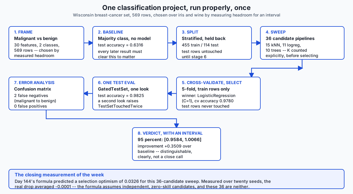
Frame states, in one sentence, what is being predicted, from what
features, and in what population. For this lesson: malignant versus
benign status, from 30 measurements taken from a fine-needle aspirate, in
the population represented by the 569 rows of load_breast_cancer.
Baseline is the score of the simplest possible non-model: predict the majority class every time. Here, 0.6316 — 357 of 569 rows are benign, so guessing benign every time gets you 63.16 percent right for free.
Split divides the 569 rows into 455 training rows and 114 test rows, stratified so the malignant/benign ratio matches in both halves, with the test rows held back from everything until stage six.
Sweep and cross-validate builds K = 36 candidate pipelines — 15
values of k for k-nearest-neighbours, 11 values of the regularisation
strength C for logistic regression, 10 values of max_depth for a
decision tree — and scores every one of them with 5-fold stratified
cross-validation on the 455 training rows. No candidate ever sees a test
row during this stage.
Select picks the highest-scoring candidate: LogisticRegression(C=1),
at a cross-validated accuracy of 0.9780.
One test evaluation fits that winning configuration on the full 455 training rows and scores it, exactly once, against the 114 held-back rows, wrapped in a gate that refuses a second look. The result: 0.9825.
Error analysis opens the confusion matrix rather than stopping at the accuracy number, and finds two false negatives (malignant predicted benign) and zero false positives.
Verdict states a 95 percent interval around the test score —
[0.9584, 1.0066] — and compares the 0.3509 improvement over baseline
against that interval’s 0.0241 half-width, concluding the model is
clearly distinguishable from guessing.
Now the things this exercise is not.
It is not a demonstration that the selection-optimism formula was wrong. Day 144 measured that formula on candidates engineered to be literal coin flips, and it held there — the measured optimism tracked the predicted expected maximum of K normals within 0.2 standard errors at every K tried. Today’s formula still describes exactly what it was built to describe. What today shows is that the formula’s assumptions — independence between candidates, zero true skill difference — are not free assumptions, and a sweep of real, correlated, genuinely skilled candidates does not automatically satisfy them.
It is not evidence that model selection is safe to skip checking. The measured optimism here happened to be small. Day 144 already measured a case — literal coin flips — where it was large: 0.0728 at K = 1000. The lesson of running both is not “optimism is usually small.” It is “you cannot know the size without measuring it on your own project,” which is precisely why exercise 7 in today’s lab computes the prediction and exercise 7b measures the reality, rather than either one alone.
And it is not a clinical tool. A 98.25 percent accuracy on a seventy-year-old teaching dataset, evaluated once on 114 rows, is a pedagogical result about a modelling protocol. Reading it as evidence about how well machine learning diagnoses cancer would be exactly the kind of unjustified leap this whole course has tried to train you out of making.
Why it was created and what problems it solves
Each of today’s eight stages exists because a specific, nameable failure happens when it is skipped, and every one of those failures has already been measured this week — today’s contribution is showing that they compound, in order, in one real pipeline, rather than showing any of them for the first time.
Skipping frame and baseline produces a number with no reference point. A model that reports “82 percent accuracy” sounds impressive until you learn the majority class is 81 percent of the data — Day 141’s whole argument, that a score means nothing without knowing what it beats.
Skipping the split, or splitting after fitting something, is Day 143’s stage-ordering failure: a scaler, a feature selector, or a hyperparameter search that has seen test rows leaks information about those rows into every downstream decision, silently and often invisibly.
Skipping cross-validation in favour of a single validation split reintroduces the holdout-variance problem Day 144 measured directly: a single split’s score can swing by 19 accuracy points across seeds on identical data. Cross-validating the 36-candidate sweep here is what makes the winner’s cross-validated score, 0.9780, a stable enough number to select on.
Skipping the accounting on how many candidates you tried is the selection-optimism problem, and today’s exercise 7 is built specifically to make you compute the prediction — 0.0326 — before you find out what actually happened. That ordering matters. Computing the prediction after seeing the answer would let you rationalise any gap; computing it first makes the −0.0001 measured result a genuine surprise rather than a retrofit.
Skipping error analysis hides exactly what today’s confusion matrix reveals: an accuracy figure is a weighted average of two different kinds of correctness, and a model can be excellent by that average while making only the costlier kind of mistake. Two false negatives and zero false positives is not visible in 0.9825 alone.
Skipping the interval turns a verdict into a guess dressed as a
fact. Day 144 built the machinery — sqrt(p(1-p)/n), the half-width
table — and today applies it to an actual decision: is 0.9825 meaningfully
better than 0.6316, given only 114 test rows? The interval says yes,
decisively. It could easily have said no, on a smaller test set or a
smaller improvement, which is exactly why the arithmetic is run rather
than assumed.
And skipping the discipline that keeps the test set honest — using it to select rather than to confirm — is the mistake exercise 10 reconstructs directly. It is, in the applied-ML literature and in real teams, probably the single most common way a reported number ends up inflated: not a dramatic leak, just quietly trying several models against the number you eventually report and keeping whichever one looked best.
How it works
Choosing the dataset, by measuring
Three classification datasets ship inside scikit-learn and need no
download: load_iris, load_wine, and load_breast_cancer. This lesson
tried all three, measured them, and rejected two.
| dataset | rows | features | classes | majority baseline | test rows at 20% |
|---|---|---|---|---|---|
| iris | 150 | 4 | 3 | 0.3333 | 30 |
| wine | 178 | 13 | 3 | 0.3889 | 36 |
| breast_cancer | 569 | 30 | 2 | 0.6316 | 114 |
With this lesson’s 36-candidate sweep, iris and wine both saturate
near-perfect cross-validated accuracy, and their test sets — 30 and 36
rows — are coarse: one wrong answer moves accuracy by more than two and
a half points. That is too blunt an instrument to compute an honest
interval, and too blunt to see selection optimism behave the way Day
144’s theory predicts, because the winning candidate’s true accuracy and
its measured accuracy on 30 rows are nearly indistinguishable from noise
in either direction. breast_cancer gives 114 test rows — still not
huge, but enough for a half-width of ±0.0241 rather than ±0.09 — and a
baseline, 0.6316, that is not trivially beaten. That headroom is why this
lesson uses it.
The frame, and the baseline
The frame is one sentence: predict malignant versus benign from 30
real-valued measurements. The baseline is one function call —
DummyClassifier(strategy="most_frequent") — fitted on the training
rows and scored on the held-back test rows: 0.6316. Every later number in
this lesson is read against that figure.
The split
train_test_split(X, y, test_size=0.2, random_state=0, stratify=y) gives
455 training rows and 114 test rows, with the malignant/benign ratio
preserved in both halves to within 1 percentage point. From this line
onward, x_test and y_test are not touched again until stage six.
The sweep
Thirty-six candidate pipelines, built with scikit-learn’s Pipeline so
that any preprocessing (here, StandardScaler ahead of the distance- and
gradient-based estimators) is refit inside every cross-validation fold
rather than fitted once on everything — Day 143’s ordering rule, now
enforced by the estimator’s own contract rather than by discipline alone:
from sklearn.pipeline import Pipeline
from sklearn.preprocessing import StandardScaler
from sklearn.neighbors import KNeighborsClassifier
from sklearn.linear_model import LogisticRegression
from sklearn.tree import DecisionTreeClassifier

configs = []
for k in range(1, 16):
    configs.append(("knn", k, Pipeline([
        ("scale", StandardScaler()), ("clf", KNeighborsClassifier(k)),
    ])))
for c in [0.001, 0.003, 0.01, 0.03, 0.1, 0.3, 1, 3, 10, 30, 100]:
    configs.append(("logreg", c, Pipeline([
        ("scale", StandardScaler()), ("clf", LogisticRegression(C=c, max_iter=5000)),
    ])))
for depth in range(1, 11):
    configs.append(("tree", depth, Pipeline([
        ("clf", DecisionTreeClassifier(max_depth=depth, random_state=0)),
    ])))
That is K = 36, counted, not estimated. Day 144’s whole complaint about selection optimism was that K is “the number nobody remembers” — this lesson remembers it because the code that builds the sweep is also the code that counts it.
Cross-validate, then select
Every one of the 36 candidates is scored with 5-fold stratified cross-validation on the 455 training rows, and the highest mean wins:
from sklearn.model_selection import StratifiedKFold, cross_val_score

splitter = StratifiedKFold(n_splits=5, shuffle=True, random_state=0)
scored = [
    (family, param, cross_val_score(make(), x_train, y_train, cv=splitter).mean())
    for family, param, make in configs
]
scored.sort(key=lambda row: -row[2])
winner_family, winner_param, winner_cv = scored[0]
The winner: LogisticRegression(C=1), cross-validated accuracy 0.9780.
Nothing in this stage has read x_test or y_test.
The predicted optimism, computed before the answer is known
Day 144’s formula, applied here, before stage six runs: the standard error of an accuracy measured on one cross-validation fold’s worth of rows (91, since 455 divided by 5 folds is 91), times the expected maximum of K = 36 standard normal draws.
se = sqrt(0.978 * (1 - 0.978) / 91) = 0.0154
expected_max_of_normals(36) = 2.118
predicted optimism = 0.0154 * 2.118 = 0.0326
That is the number to write down before looking at the test set. It says: “if these 36 candidates behave like Day 144’s coin flips, expect the cross-validated score to overstate the real accuracy by about three points.”
One test evaluation, gated
class GatedTestSet:
    def __init__(self, X, y):
        self._X, self._y, self.evaluations = X, y, 0

    def evaluate(self, model):
        if self.evaluations >= 1:
            raise TestSetTouchedTwice(
                "the test set has already been used once; any further "
                "score is a validation score, not a test score"
            )
        self.evaluations += 1
        return float(model.score(self._X, self._y))
Fitting the winner on the full 455 training rows and calling
gate.evaluate(fitted) once gives 0.9825. A second call raises. The
measured drop — cross-validated minus test — is 0.9780 - 0.9825 = -0.0045. The test score came out slightly better than the
cross-validated one, not worse: the opposite sign from what the
predicted optimism implied.
Predicted versus measured, over twenty seeds
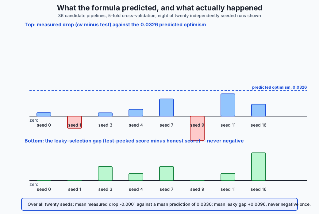
One seed is an anecdote — Day 144’s own reporting rule, applied here. The same measurement, repeated at seeds 0 through 19:
| quantity | predicted (mean) | measured (mean) | measured (sd) |
|---|---|---|---|
| selection optimism | 0.0330 | −0.0001 | 0.0149 |
Read that pair carefully. The prediction is consistently around 0.033 at every seed — it barely moves, because it depends mostly on K and the fold size, both fixed. The measurement is centred almost exactly on zero, and it is noisy in both directions: at some seeds the drop is positive (the model looked worse on test than on cross-validation), at others negative (it looked better), roughly half and half. The formula predicted a one-sided inflation; reality gave a two-sided scatter around zero.
Why the formula overestimates here
Two facts about this sweep break the formula’s assumptions, and both are worth internalising because they generalise to almost any real hyperparameter sweep you will ever run.
The candidates are correlated, not independent. Day 144’s formula
assumes K independent noisy estimates — the maximum of K genuinely
separate coin flips. But KNeighborsClassifier(4) and
KNeighborsClassifier(5) make nearly identical predictions on nearly
identical rows; so do LogisticRegression(C=1) and
LogisticRegression(C=3). The effective number of independent choices
in this sweep is far smaller than 36, and a smaller effective K means a
smaller expected maximum — and therefore less optimism than the formula,
which used the nominal K = 36, predicts.
The candidates have genuine, if small, skill differences. Day 144’s
coin-flip candidates were constructed to have exactly zero true skill, so
every difference between them was pure noise, and picking the “best” one
was picking the luckiest one. Here, some configurations genuinely
generalise better than others — LogisticRegression(C=1) is not luckier
than DecisionTreeClassifier(max_depth=1), it is a better-suited model
for this problem. Selecting the best cross-validated score is picking up
some of that real signal along with some noise, and the noise component —
the only part the formula is describing — is a smaller share of the
total than it was for candidates with zero true skill.
Neither of these facts makes the check unnecessary. They make it a check you have to run on your own sweep, because you cannot know in advance how correlated your candidates are or how much real skill separates them.
Error analysis: what the confusion matrix says
The one test evaluation’s predictions, compared against the true labels:
             predicted
             malignant  benign
true malignant    40       2
true benign        0      72
Two malignant cases predicted benign — false negatives, in the sense that matters here: a real cancer the model said was not one. Zero benign cases predicted malignant. An accuracy of 0.9825 does not distinguish “the model makes two false negatives and zero false positives” from “the model makes one of each” — those are the same accuracy, and a very different error profile. In a screening context, a missed malignancy is generally the costlier mistake — it delays treatment, where a false alarm merely triggers a follow-up test. Reading the matrix, not just the accuracy, is what tells you which kind of mistake you are actually making.
The verdict, with an interval
n_test = 114
se = sqrt(0.9825 * (1 - 0.9825) / 114) = 0.0123
half-width (95%) = 1.96 * 0.0123 = 0.0241
interval = [0.9584, 1.0066]
improvement over baseline = 0.9825 - 0.6316 = 0.3509
0.3509 is roughly fourteen times the interval’s half-width. This is not a “cannot distinguish” case — Day 144’s cautionary tale about small test sets does not bind here, because the improvement is enormous relative to the noise. It could easily have gone the other way: if the improvement had been 0.015 rather than 0.35, the interval would have swallowed it whole, and the honest verdict would have been “cannot distinguish this model from guessing at this test-set size.” Computing the interval, every time, is how you find out which case you are in rather than assuming.
The leaky version, run alongside the honest one
Exercise 10 reconstructs, deliberately, the mistake this whole course has spent nine days building discipline against: selecting a model by fitting every candidate and scoring each one directly on the test set, rather than selecting on cross-validated training rows and looking at test once.
def leaky_selection_test_score(x_train, y_train, x_test, y_test):
    best = -1.0
    for _family, _param, make in configs:
        pipe = make().fit(x_train, y_train)
        best = max(best, pipe.score(x_test, y_test))
    return best
At the headline seed, the leaky score and the honest score tie: both 0.9825, a gap of exactly zero. That is a ceiling effect — 114 test rows mean accuracy can only move in steps of about 0.0088, so ties are common. Over twenty seeds, the mean gap is +0.0096 (standard deviation 0.0103, maximum 0.0351), and — this is the structural fact worth remembering — it is never negative, at any seed tried. The leaky search considers the honest winner among its 36 candidates and can only replace it with something that scored at least as well on the very rows it was allowed to peek at. It cannot lose. It can only tie or win, which is not luck — it is the mechanism.
An everyday analogy
A university admissions committee reviewing one applicant’s file.
Baseline is what you would predict about the applicant knowing nothing but the overall acceptance rate — say, admit rates run around 60 percent at this school, so guessing “admit” for everyone gets you 60 percent right with zero effort.
The frame is deciding, precisely, what you are predicting: not “is this a good person” but “will this student succeed in our specific program, based on this specific application.”
The split is deciding, before reading the file, which parts of the record inform the committee’s deliberation (transcripts, essays, recommendations — read as many times as needed) and which part is held back for a final check (say, a single reference call made once, after the decision, purely to confirm nothing was missed — never to change the decision).
The sweep is the committee trying several different weighting schemes for the file — weight test scores heavily, weight essays heavily, weight extracurriculars heavily — and scoring each scheme against past applicants whose outcomes are already known.
Cross-validation is checking each weighting scheme against several different subsets of those past applicants, not just one, so a scheme that happened to work well on one arbitrary subset of history does not get crowned the winner by luck.
Selection is the committee agreeing on one weighting scheme — the one that did best across those checks.
The one look is applying that agreed-upon scheme to the actual applicant’s actual file, once, and reaching a decision. Not re-weighting after seeing how the applicant “would have scored” under six different schemes and picking whichever gives the answer the committee already wanted.
Error analysis is not stopping at “we admit roughly the right fraction of students” — it is checking whether the mistakes cluster: are you disproportionately rejecting strong candidates from one background, or disproportionately admitting weak candidates from another? That question is invisible in an overall accept rate.
The verdict is not “we’re pretty confident in this decision.” It is “here is our historical error rate on decisions like this one, and here is the range that error rate plausibly falls in, given how many past decisions we actually reviewed.”
The analogy earns its keep on the leaky-selection failure. Imagine a committee member who, instead of trusting the pre-agreed weighting scheme, quietly tries all six schemes on this specific applicant and recommends whichever one produces the admission decision they already favoured — then reports “our scheme recommended admit” as though it were the pre-agreed process speaking. That report can never look worse than the honest process, and it will often look identically confident, because from the outside “admit” is “admit” regardless of which of six schemes produced it. The dishonesty is invisible in the recommendation itself; it lives entirely in which of six numbers got reported after the fact.
Examples in practice
A learner who stops at 98.25 percent
The most common mistake this lesson is built to correct: a project that reports “98.25 percent accuracy” and nothing else. Two follow-up questions immediately matter. Ninety-eight point two five percent of what — a baseline of 63 percent, or a baseline of 98 percent, where the same score would mean the model learned nothing at all? And what kind of two percent is wrong — evenly split errors, or all of one costly type? Both questions have concrete answers here (0.6316 and “two false negatives, zero false positives”) and neither is visible in the headline number alone.
A team that tunes against its own test set without noticing
The most common real instance of exercise 10’s leaky version rarely looks
like a single dramatic mistake. It looks like a team that has one
official test set, tries a model, checks the test score “just to see,”
tries a tweak, checks again, tries another tweak, checks again — and
after the fifth check, reports the best one as “our result.” No single
check felt like cheating. The cumulative effect is exactly
leaky_selection_test_score: K looks at the test set disguised as one.
The fix is not vigilance — it is a GatedTestSet that makes the sixth
look impossible rather than merely inadvisable.
A model comparison that never sizes its test set
An engineer is asked whether a new model beats the old one by two points. Before touching any code: at an accuracy near 0.85, resolving a two-point difference at 95 percent confidence needs 1225 test rows — Day 144’s sizing table, arriving at an actual decision. If only 400 rows are labelled, the interval is roughly ±0.035, wider than the difference being chased, and the honest answer is “this comparison cannot be made with the data we have,” delivered before a single model is trained.
Reading a published benchmark’s confusion matrix, not just its headline
A paper reports “97 percent accuracy on cancer detection.” The number alone answers almost nothing useful. Which of the two classes does the 3 percent of errors fall into? On a dataset where malignant cases are the minority, a model that is excellent at recognising benign cases and mediocre at recognising malignant ones can post a high accuracy while being clinically closer to useless — exactly the asymmetry this lesson’s confusion matrix makes visible and a bare accuracy figure hides.
Implications: security, privacy, performance, scalability, and cost
The cost of skipping a baseline is a project that never gets challenged. A model reporting 82 percent on a dataset that is 81 percent one class will pass every casual review, because 82 percent sounds good. The baseline is a one-line, zero-cost check that catches this before anyone spends a week building on top of it.
The cost of a leaky selection is a number that fails in production and
nowhere else. Every metric a team reports internally can look
consistent and healthy right up until deployment, because the leak lives
entirely in how the number was produced, not in any property of the data
that a dashboard could flag. GatedTestSet is a cheap, mechanical defence
against exactly this — one object, refusing a second call, costs nothing
to add and closes the most common real-world version of this mistake.
Error analysis is a security and safety control, not a nicety. A false negative in fraud detection is a fraudulent transaction that goes through; a false positive is a legitimate customer inconvenienced. Those have wildly different costs, and a system tuned to overall accuracy alone can quietly optimise for the wrong one. Today’s confusion matrix, applied to a domain where the asymmetry is worse than a two-by-two table can fully convey, is the minimum bar for catching this before deployment.
Computing the predicted optimism costs nothing and catches a lot.
se * expected_max_of_normals(K) is two function calls, run before the
test set is touched. On a sweep where the prediction turns out to matter —
unlike this lesson’s, where it did not — that arithmetic is the
difference between reporting a real number and reporting an artefact of
how many things you tried.
Cross-validating 36 candidates costs 36 times 5 model fits, which is cheap here and would not be on a larger model. The trade-off Day 144 named — compute against a nineteen-point swing on a single holdout — is this lesson’s trade-off too: on a laptop-scale sweep like this one, the extra compute is not a close call. On a sweep of expensive models, the right answer shifts to a single holdout reported with an interval, never to skipping the check.
And the largest, least visible cost is a project that never runs the selection-optimism check because it “obviously doesn’t matter here.” This lesson’s own result — the check mattered enough to overturn a prediction that would otherwise have gone unquestioned into a report — is the argument against skipping it, not evidence that it can safely be skipped from now on.
Alternatives: free, open source, and commercial
scikit-learn’s own protocol tools — used throughout this lesson
When to choose them: for essentially all in-memory classification
work. Every stage of today’s protocol — Pipeline, StratifiedKFold,
cross_val_score, DummyClassifier, confusion_matrix — is free,
BSD-3-Clause or MIT licensed, with no paid tier, and every number in this
lesson comes from them.
How to use them: chained together exactly as shown in “How it
works” — a Pipeline per candidate, cross_val_score per sweep,
confusion_matrix for error analysis, and a hand-rolled
sqrt(p*(1-p)/n) for the interval, since scikit-learn does not ship an
interval helper for accuracy directly.
Watch for: Pipeline protects you from leaking a fitted transform
across the train/test boundary, but it does not protect you from leaking
the test set itself into selection — exercise 10’s mistake happens
entirely outside any estimator’s contract, in how you choose to call
.score().
GridSearchCV and RandomizedSearchCV — described, not used here
When to choose them: when the sweep is large enough that writing the
candidate loop by hand becomes unwieldy, or when you want randomised
sampling over a continuous hyperparameter space rather than a fixed grid.
Both are free, built into scikit-learn, and functionally equivalent to
today’s hand-written sweep-and-select loop — GridSearchCV would have
produced the same winner from the same 36 candidates.
What they add: parallel fitting across candidates and folds via
n_jobs, and a .best_estimator_ attribute that saves you the manual
bookkeeping this lesson’s select_best does by hand.
Honest note: this lesson writes the sweep manually specifically so
every step — counting K, cross-validating, comparing predicted to
measured optimism — stays visible rather than living inside a library
call. GridSearchCV is the right tool once you trust the process; today
is about building that trust.
Nested cross-validation — the theoretically correct fix, described
When to choose it: when you must both select a model and produce an honest estimate of how well the selected model generalises, using the same limited data, without a separate untouched test set at all. An inner cross-validation loop selects; an outer loop scores the winner of each inner selection, so the outer score is never contaminated by the selection that produced it.
What it costs: the product of the two loops — five inner folds times five outer folds is 25 times the fits of a single cross-validation pass.
Honest note: this lesson’s lab does not implement nested cross-validation; it is named here and left as an extension exercise, because this lesson already has a genuine held-out test set and does not need nested CV to get an honest estimate — nested CV earns its complexity specifically when a separate test set is not affordable.
Managed experiment-tracking platforms — not used here
The relevant capability for this lesson: the same one Day 144 named — they can tell you K, the number of configurations actually tried against a given metric, which is precisely the number this lesson’s exercise 7 had to count by hand from the sweep’s own source code.
Free versus paid: most offer a free tier for individual use and charge for team features; no specific price is quoted here, because pricing changes faster than this lesson does, and an unverified figure is worse than none. Free, self-hosted, open-source options exist and log the same information.
Comparison with related concepts
| Concept | What it does | How it relates to today |
|---|---|---|
| A single train/test split | one division, one score | What this lesson’s split stage builds on, and what cross-validation replaces for selection |
| Cross-validation | every training row tests exactly once | Used here to select among 36 candidates without ever touching test rows |
| Selection-optimism formula | predicts inflation from K and the validation standard error | Applied here, and found to overestimate the real effect by roughly thirty-fold, for reasons this lesson explains |
| Nested cross-validation | an inner loop selects, an outer loop scores | The theoretically correct alternative to a held-out test set; not needed here because a real test set exists, described as an extension |
| Confusion matrix | predicted class against true class | This lesson’s error-analysis stage; reveals the false-negative/false-positive split an accuracy figure hides |
| A 95 percent interval on accuracy | quantifies how much a test score could plausibly move | This lesson’s verdict stage, applied to an actual pass/fail decision about the model |
| Leaky selection | choosing a model by scoring it on the test set | Deliberately reconstructed in exercise 10, to show the never-negative asymmetry directly rather than only in the abstract |
| GatedTestSet | mechanically enforces one test evaluation | Reused unchanged from Day 144, protecting the real test rows of a real project |
Two rows deserve a closing note.
The selection-optimism formula row is the whole week’s thesis in miniature. It is not “always trust the formula” and it is not “the formula is wrong and can be ignored.” It is: compute the prediction, measure the reality, and report whichever one the data actually supports — which is what exercises 7 and 7b, run in that order, force you to do.
And the leaky-selection row is the mistake most likely to happen to
you specifically, more than group leakage or temporal leakage, because
it requires no unusual data structure — just checking the test score one
extra time. GatedTestSet exists because good intentions are not a
reliable enough defence against a mistake this easy to make by accident.
When to use it — and when not to
Run the full eight-stage protocol whenever a model’s result will inform a real decision — a deployment, a publication, a comparison against a baseline someone will act on. The cost is one afternoon and a handful of extra function calls; the alternative cost, when this protocol is skipped, is a number that fails exactly when it matters most, in production or in front of a reviewer.
Compute the predicted selection optimism before every real sweep, not only when you suspect it will matter. This lesson’s own headline result — a case where the naive prediction badly overestimated reality — was only discoverable because the check was run rather than assumed unnecessary.
Open the confusion matrix whenever the classes carry different real costs, which is most classification problems worth building. An overall accuracy figure treats a false positive and a false negative as interchangeable; almost no real domain does.
Compute the test-set interval before treating any comparison as settled. An improvement smaller than the interval’s half-width is not evidence of anything, however good the point estimate looks.
And use GatedTestSet, or an equivalent, whenever more than one person
or more than one script can reach the test set — the leaky-selection
mistake this lesson reconstructs almost never happens on purpose.
When the full protocol is more than the situation needs: a genuinely exploratory first look at brand-new data, where nothing will be reported or deployed and the goal is purely to build intuition, can reasonably skip the formal split-and-gate machinery — provided nobody later reuses that exploratory number as though it were a validated result. The moment a number leaves the exploratory phase and starts informing a decision, the full protocol applies.
The AI thread
Every stage of today’s protocol gets harder, not easier, at the scale modern AI systems operate at, and the selection-optimism finding is the sharpest version of why.
The number of “candidates” in a large model’s development is uncountable, and the naive formula would be catastrophically wrong in the other direction. A frontier model’s final configuration is typically the survivor of an enormous, informally tracked search across architectures, data mixtures, and training recipes — a K that is not 36 but plausibly in the thousands, spread across a team and a timeline nobody fully reconstructs. Unlike this lesson’s sweep, where correlated, skilled candidates made the real optimism smaller than a naive K=36 formula predicts, an uncounted, genuinely enormous K in an industrial search makes the true optimism potentially far larger than anyone reports — and there is no equivalent of exercise 7b to check it against, because there is rarely a truly held-out test set that nobody on the team has ever looked at.
Public benchmark leaderboards are exactly the leaky-selection failure, at planetary scale. Every team that submits a model to a public leaderboard and iterates based on the score is running exercise 10’s mistake — selecting using the “test” set — except the leaderboard is shared across thousands of teams over years, so the effective K is uncountable and the resulting inflation, unlike this lesson’s small measured gap, has in some documented cases been substantial when fresh test data was collected.
And the confusion-matrix discipline matters more, not less, as models get deployed into higher-stakes decisions. A large language model graded on overall “helpfulness” or “accuracy” can hide the same asymmetry this lesson’s malignant/benign matrix makes visible — a model can be excellent on average while being reliably wrong on a specific, costly category of input, and an aggregate score will never show you that category exists. The discipline this lesson teaches at the scale of one confusion matrix and 114 rows is the same discipline that has to scale to systems evaluated on millions of interactions: never trust the average without asking what the errors are made of.
Knowledge check
candidate_summaries()shows iris and wine saturating near-perfect cross-validated accuracy with a 36-candidate sweep, while breast_cancer does not. Explain, in terms of test-set size and accuracy ceiling, why that made iris and wine unsuitable for this lesson’s exercises.- Day 144’s formula predicts a selection optimism of 0.0326 for this lesson’s sweep. The measured mean drop over twenty seeds is −0.0001. Name the two properties of this sweep’s 36 candidates that explain the gap, and say why neither property held for Day 144’s coin-flip candidates.
- The confusion matrix is
[[40, 2], [0, 72]]at an overall accuracy of 0.9825. Explain what specific fact this matrix reveals that the accuracy number alone does not. - The 95 percent interval around the test accuracy is
[0.9584, 1.0066], and the improvement over baseline is +0.3509. State the rule connecting these two numbers to the verdict, and describe a hypothetical improvement size that would have forced a “cannot distinguish” verdict instead. - In exercise 10, the leaky-selection gap is sometimes exactly zero but never negative, across twenty seeds. Explain the mechanism that makes a negative gap impossible, and explain separately why a gap of exactly zero is unsurprising given the test set has only 114 rows.
- A learner concludes: “Selection optimism turned out to be nearly zero in this lesson, so I don’t need to check it on my own project.” Explain what is wrong with that reasoning, using Day 144’s own coin-flip measurement as a counter-example.
- State, in order, the eight stages of this lesson’s protocol, and name one specific measured failure from Days 141-144 that each stage defends against.
- Why does this lesson compute the predicted selection optimism (exercise 7) before measuring the actual drop (exercise 7b), rather than the other way around?
Hands-on exercise
Today’s lab, One Classification Project, Run Properly, runs the entire
eight-stage protocol on the Wisconsin breast-cancer dataset and asks you
to verify every measured number along the way.
Fourteen exercises. The first four establish the dataset choice, the baseline, the split and the sweep. The next three build the cross-validated selection, the gated one-time test evaluation, and the predicted-versus-measured selection optimism — the closing result of the week. The last four cover error analysis, the interval-based verdict, and the leaky-selection reconstruction.
Build the environment, then work through
starter/test_classification_claims.py, replacing one pytest.skip at a
time.
Expected output
The harness ends with:
---------------------------------------------------------------
15 checks, 0 failure(s)
and exits 0. pytest examples -q reports 18 passed, and
pytest starter -q reports 4 passed, 14 skipped until you begin.
The measured table includes:
  K = 36 candidate pipelines: 15 KNN, 11 logistic regression, 10 decision trees
  winner: logreg (1)  5-fold CV accuracy = 0.9780
  test accuracy: 0.9825
  predicted optimism (SE of a CV fold x expected max of 36 normals): 0.0326
  mean measured drop: -0.0001  sd 0.0149
  confusion matrix: [40, 2] / [0, 72]
  false negatives (malignant predicted benign): 2
  95 percent interval: [0.9584, 1.0066]
  mean leaky gap: +0.0096  fraction of seeds where the leak was non-negative: 1.0000
Validate your work
bash tests/run_tests.sh; echo "exit=$?"reports15 checks, 0 failure(s)andexit=0. Capture the harness’s own exit status..venv/bin/pytest examples -qreports18 passed..venv/bin/python3 examples/report_measurements.py | diff - expected-output/measured-values.txtproduces no output.- When you have finished every exercise,
pytest starter -qreports18 passed. - Break one assertion on purpose, confirm the harness fails, restore it.
Troubleshooting
The harness takes a while. Exercises 7b and 10b each cross-validate 36 candidates across 20 seeds — 720 five-fold cross-validations apiece. No timing is asserted, so a slow machine changes nothing about whether it passes.
My winning configuration differs from the lesson’s. Check
expected-output/FIELDS.md. Several configurations score within a point
or two of LogisticRegression(C=1), and different NumPy or scikit-learn
versions can legitimately shuffle a tie differently — Day 145 already
established that near-tied configurations trade places under resampling.
The predicted optimism doesn’t match my by-hand calculation.
predicted_selection_optimism uses the size of one cross-validation
fold (455 divided by 5, giving 91), not the full training set, because
that is the number of rows each fold’s held-out score is actually
computed from.
My leaky-gap numbers differ from the lesson’s. Almost certainly fine if a single seed’s gap is zero — a ceiling effect from only 114 test rows. What must hold across the full 20-seed sweep is that the gap is never negative.
import file mismatch. You ran pytest examples starter together.
Run them separately.
Common mistakes
Reporting the test accuracy without the interval. A point estimate with no half-width is not a verdict, and this lesson’s own comparison — 0.3509 improvement against a 0.0241 half-width — would have looked very different at a smaller improvement or a smaller test set.
Treating the small measured selection optimism as proof the check is unnecessary. Day 144 already measured a case where it was not small. The check tells you which case you are in; skipping it assumes the answer.
Reading 0.9825 accuracy without opening the confusion matrix. The two errors this model makes are not interchangeable, and the accuracy figure alone cannot tell you that.
Concluding the leaky-selection gap is “basically zero and therefore harmless.” The gap is small at any one seed partly because of the test set’s coarse granularity, but it is never negative across twenty seeds — the mechanism, not the size, is the point.
Practice assignment
Take a classification result you already have — from a project, a tutorial, or your own experiments — and run this lesson’s protocol against it, honestly.
- State your baseline. What does the majority class get you for free? If you cannot answer this in one line, your project has not been framed yet.
- Count your K. How many models, hyperparameters, or feature sets were tried against whatever number you are about to report? Estimate it honestly, in writing, even if the true count is embarrassing.
- Compute the predicted optimism, using your validation set’s standard error and your counted K, and compare it to whatever improvement you are claiming.
- Measure the real gap, if you can. If you have a genuinely untouched holdout, compare your cross-validated score to a single evaluation on it. If you do not have one, say so plainly — that is a finding too.
- Open your confusion matrix, and name which of your errors is costlier in your actual domain, not just which is more frequent.
- State your verdict as an interval, and say explicitly whether your claimed improvement clears it.
The deliverable is the audit, in writing, not a better model.
Extension challenge
Pick one and measure it.
- Nested cross-validation. Implement an inner selection loop and an outer scoring loop, and measure whether the gap between cross-validated and outer-scored accuracy shrinks further than this lesson’s single test evaluation showed. Report the cost in fits.
- A fourth candidate family. Add support-vector classifiers to the sweep, re-run the full protocol, and report whether the winner or its cross-validated score changes at the headline seed.
- Cost-weighted error analysis. Assign an explicit cost to a false negative versus a false positive — say, ten to one — and determine whether a different candidate from the 36-model sweep would have been preferred under that weighting.
- Scale the test set and re-measure the leaky gap. Repeat the leaky-vs-honest comparison with a 60/40 train/test split instead of 80/20, so the test set holds roughly 227 rows instead of 114, and report whether the mean gap and its granularity both change as predicted.
- Break independence on purpose. Duplicate a fraction of the rows into both the train and test splits before running the sweep, and measure how much the reported test accuracy inflates — Day 144’s group-leakage lesson, reconstructed on real data instead of a synthetic one.
- Find the break-even K for this dataset. At what number of correlated, real candidates would the predicted optimism formula and the measured reality actually agree? Vary the sweep’s composition — more independent model families, fewer near-duplicate hyperparameters — and report what changes the answer.
Quiz
Q1. Iris and wine both ship inside scikit-learn, need no download, and are the classic teaching datasets. This lesson uses breast_cancer instead. Why, specifically?
- A 36-candidate sweep saturates near-ceiling accuracy on iris and wine, and their 30-36 test rows are too coarse for an honest interval or a meaningful selection-optimism check
- Breast_cancer is a binary classification problem and iris and wine are not, and this lesson only covers binary classification
- Iris and wine are not free to use commercially, unlike breast_cancer
- Breast_cancer has more features, and more features always make a better teaching example
Show answer
Answer: A. A 36-candidate sweep saturates near-ceiling accuracy on iris and wine, and their 30-36 test rows are too coarse for an honest interval or a meaningful selection-optimism check
candidate_summaries() measures all three: iris and wine both saturate near-perfect cross-validated accuracy with this lesson's 36 candidates, and their test sets (30 and 36 rows) move accuracy in steps of roughly 3 points -- too coarse to support the interval and selection-optimism work this lesson does. breast_cancer's 569 rows and 114-row test set give room for both. All three datasets are bundled and free; the class-count claim about "only binary" is simply false, since nothing about the protocol in this lesson requires two classes.
Q2. Day 144's formula predicts a selection optimism of 0.0326 for this lesson's 36-candidate sweep. The measured drop at the reported seed is -0.0045, and the mean measured drop over 20 seeds is -0.0001. What is the correct reading of this gap?
- The formula is wrong and should be discarded for real projects
- The formula assumes independent, zero-skill candidates; these 36 are correlated (adjacent hyperparameters behave almost identically) and genuinely skilled, so it overestimates the real optimism here
- The measurement is wrong, since theory should always match practice exactly
- Selection optimism only applies to classification, not regression, which is why it did not appear
Show answer
Answer: B. The formula assumes independent, zero-skill candidates; these 36 are correlated (adjacent hyperparameters behave almost identically) and genuinely skilled, so it overestimates the real optimism here
The formula's derivation assumes K independent draws with no true skill difference between them -- literally what Day 144's coin-flip candidates were. This lesson's 36 candidates are neither: nearby k values and nearby regularisation strengths make almost identical predictions, so the effective number of independent choices is far below 36, and every candidate carries real skill rather than being pure noise. The formula still correctly signals that some optimism check is warranted; it simply is not calibrated for this kind of correlated, skilled sweep, and the honest response is to measure the real gap rather than trust either the formula or a single seed.
Q3. The confusion matrix for the winning model is [[40, 2], [0, 72]] (rows true, columns predicted, order malignant then benign), at an overall accuracy of 0.9825. What does the accuracy figure alone fail to tell you?
- That the model achieved above-baseline performance at all
- The total number of test rows used to compute it
- That both of the model's two errors are false negatives -- malignant cases predicted benign, the clinically costlier mistake -- while zero benign cases are misclassified as malignant
- Whether the model was trained using cross-validation
Show answer
Answer: C. That both of the model's two errors are false negatives -- malignant cases predicted benign, the clinically costlier mistake -- while zero benign cases are misclassified as malignant
A single accuracy number of 0.9825 sounds uniformly good and gives no hint that the two mistakes it represents are not interchangeable: both are false negatives, the costlier error in cancer screening because it delays treatment rather than triggering an unnecessary follow-up. The other three options are either recoverable from the accuracy figure and n_test directly, or are facts about the training procedure that the confusion matrix does not encode either.
Q4. The test set has 114 rows. The 95 percent interval around the test accuracy of 0.9825 is [0.9584, 1.0066], and the improvement over the 0.6316 baseline is +0.3509. What is the correct verdict?
- Cannot distinguish the model from the baseline, because the interval crosses above 1.0, which is impossible for an accuracy
- No verdict is possible until the test set is evaluated a second time to confirm the result
- The model is overfitting, because 0.9825 is close to a perfect score
- The improvement is clearly distinguishable from the baseline, since 0.3509 is far larger than the interval's 0.0241 half-width
Show answer
Answer: D. The improvement is clearly distinguishable from the baseline, since 0.3509 is far larger than the interval's 0.0241 half-width
The improvement (0.3509) is roughly fourteen times the interval's half-width (0.0241), so the model is comfortably distinguishable from baseline at this test-set size -- an honest verdict this lesson could easily have come out the other way with a smaller improvement or a smaller test set, which is exactly why the interval is computed rather than assumed. The interval extending slightly above 1.0 is an artefact of the normal approximation near a boundary, not evidence of a problem, and does not change the comparison. A second test evaluation would not confirm anything -- it would be a validation score wearing the word test, per Day 144. And near-ceiling accuracy on its own says nothing about overfitting without comparing train and validation behaviour, which Day 145 covered.
Q5. Exercise 10 selects a model by fitting all 36 candidates and scoring each one directly on the test set, instead of selecting on cross-validated training rows. Over 20 seeds, this leaky score is never lower than the honest score, though the gap is sometimes exactly zero. Why can the gap never be negative?
- Because the leaky search considers the honest winner among its 36 candidates and can only replace it with something that scored at least as well on the very rows it was allowed to peek at
- Because the leaky search always trains on more data than the honest one
- Because the test set is larger than the training set in this lesson
- Because logistic regression always outperforms k-nearest-neighbours on this dataset
Show answer
Answer: A. Because the leaky search considers the honest winner among its 36 candidates and can only replace it with something that scored at least as well on the very rows it was allowed to peek at
The leaky search is a superset of the honest choice: it evaluates every one of the 36 candidates, including the one cross-validation selected, directly against the test rows, and keeps whichever scores highest on those same rows. By construction it therefore cannot do worse than the honest winner's own test score -- it can only tie or improve on it, which is the exact mechanism, not chance. Training-set size is identical between the two searches, and neither family systematically wins across all 20 seeds.
Q6. 114 test rows means test accuracy can only take values that are multiples of roughly 0.0088 (1/114). What effect does this have on the leaky-selection gap measured in exercise 10b?
- None -- accuracy granularity has no bearing on whether a gap can be measured
- It is part of why the gap lands at exactly zero on some seeds: the honest and leaky searches sometimes land on the identical winner, or on winners tied at the same coarse accuracy value
- It makes the gap systematically larger than it would be with more test rows
- It means the confusion matrix cannot be computed accurately
Show answer
Answer: B. It is part of why the gap lands at exactly zero on some seeds: the honest and leaky searches sometimes land on the identical winner, or on winners tied at the same coarse accuracy value
With only 114 possible test rows, accuracy can only move in steps of about 0.0088, so two different configurations frequently tie exactly on test accuracy even if their underlying quality differs slightly -- and a tie means the leaky search has nothing to gain over the honest one at that seed, producing a gap of precisely zero. A finer-grained test set (more rows) would show a smoother, and likely more consistently positive, gap. The granularity affects the SIZE of an observable gap, not whether the confusion matrix is computable, and there is no reason it would inflate the gap.
Q7. Which of the following is the correct order for this lesson's protocol, and why does the order matter?
- Split, frame, cross-validate, fit on everything, evaluate on test as many times as needed to be sure
- Fit the best-looking model first, then decide afterward what dataset and baseline would justify it
- Frame, baseline, split, sweep and cross-validate, select, evaluate on test exactly once, analyse errors, state a verdict with an interval
- Evaluate candidates on the test set to find the best one, then cross-validate that one candidate to double-check it
Show answer
Answer: C. Frame, baseline, split, sweep and cross-validate, select, evaluate on test exactly once, analyse errors, state a verdict with an interval
Each stage in the correct order protects the next: framing and a baseline establish what "good" even means before any model exists; the split holds the test rows back; the sweep and cross-validation spend looks on training rows, where spending is free; selection happens before the one test evaluation, never after; and the verdict is stated with an interval, not a bare number. Evaluating on test repeatedly, choosing a model before framing the problem, or letting the test set do the selecting (as in exercise 10) each break a different stage of this same order, which is why this lesson measures all three as mistakes elsewhere.
Q8. A learner concludes from this lesson: "Selection optimism turned out to be nearly zero here, so checking for it was a waste of time -- I'll skip that step on my own project." What is wrong with this reasoning?
- Nothing -- if optimism is usually small, the check can reasonably be skipped
- Selection optimism is only ever nonzero when the candidates are literal coin flips, so the learner is correct in this case but the reasoning does not generalise
- The formula should have been trusted instead of the measurement, since formulas are always more reliable
- The check is how you find out whether optimism is small on YOUR project; assuming it is small because it was small on this one dataset is exactly the untested assumption the check exists to replace
Show answer
Answer: D. The check is how you find out whether optimism is small on YOUR project; assuming it is small because it was small on this one dataset is exactly the untested assumption the check exists to replace
This lesson''s own headline finding is that the closed-form prediction (0.0326) and the measured reality (-0.0001) diverged sharply -- which was only discoverable BECAUSE the check was run. A learner who skips the check on a new project because it came out small once has replaced one untested assumption (the formula always applies) with another (my optimism is always negligible), which is the same mistake in a different shape. Day 144 already showed optimism CAN be large (0.0728 on literal coin flips); this lesson shows it can also be much smaller than a formula predicts. Both are only known by measuring, on the project in front of you, every time.
Glossary
- Majority-class baseline
- The accuracy of predicting the most common class every time, with no model at all. Every model in this lesson has to clear it to be worth building -- here, 0.6316 -- and it is computed before any model is fitted, not after, as a check on whether the whole exercise is worth doing.
- Candidate pipeline
- One complete, fittable scikit-learn Pipeline -- a specific estimator with specific hyperparameters, any preprocessing folded in. This lesson sweeps 36 of them: 15 k-nearest-neighbours settings, 11 logistic-regression regularisation strengths, 10 decision-tree depths.
- K, counted
- The number of candidates actually tried in a selection sweep. Day 144 named it as the number nobody remembers; this lesson counts it explicitly at 36, because the selection-optimism formula needs it as an input.
- 5-fold stratified cross-validation
- Splitting the training rows into five class-balanced folds and scoring each candidate on all five, so every training row serves as held-out data exactly once. Used here to select the winning configuration without ever touching the test rows.
- Selection optimism, predicted
- The optimism Day 144's formula predicts for a specific sweep: the standard error of an accuracy on one cross-validation fold's worth of rows, times the expected maximum of K standard normal draws. Computed here at 0.0326 for a 36-candidate sweep, before the test set is ever consulted.
- Selection optimism, measured
- What actually happened when the prediction above was checked against a real test evaluation, over 20 independent seeds: a mean drop of -0.0001, far below the 0.0330 mean prediction, because the candidates in this sweep are correlated and genuinely skilled rather than independent and skill-free.
- GatedTestSet
- An object that wraps the held-out test rows and permits exactly one call to evaluate, raising TestSetTouchedTwice on any further attempt without advancing its own counter. The discipline from Day 144, made mechanical again on a real dataset.
- Leaky selection
- Choosing a winning configuration by fitting every candidate and scoring each one directly against the test set, instead of selecting on cross-validated training rows. Measured here at a mean gap of +0.0096 over 20 seeds, and never negative at any seed tried.
- Confusion matrix
- A table of predicted class against true class. Here, [[40, 2], [0, 72]]: two malignant cases predicted benign, zero benign cases predicted malignant -- a fact that a single accuracy number does not reveal on its own.
- False negative, in this domain
- A malignant case predicted benign -- the costlier of the two possible mistakes in cancer screening, because it delays treatment rather than triggering an unnecessary follow-up. This lesson's model makes two of them and zero of the other kind.
- 95 percent interval, on a test accuracy
- test_accuracy plus or minus 1.96 times the standard error sqrt(p(1-p)/n). Computed here at 0.9825 +/- 0.0241, giving [0.9584, 1.0066] -- the range Day 144's arithmetic says the true accuracy plausibly sits in, given only 114 test rows.
- Distinguishable from baseline
- Whether an improvement over the baseline exceeds the test set's own 95 percent half-width. Here, an improvement of 0.3509 against a half-width of 0.0241 is clearly distinguishable; a smaller improvement on the same test set might not have been, and the arithmetic is how you would find out.
- Frame
- Stating what is being predicted, from what, and what beating it would even mean, before any code is written. The first stage of this lesson's protocol, and the one skipped most often in practice.
- Verdict
- The end product of a properly run classification project: a test score, an interval around it, a statement of whether it clears the baseline given that interval, and an honest account of the specific errors the model makes -- not a single accuracy number quoted alone.
- Winner's curse, applied to a real sweep
- The same argmax-over-noisy-estimates mechanism Day 142 and Day 144 measured on bandit arms and coin flips, checked here against real, skilled, correlated candidates -- and found to overestimate the real effect by roughly thirty-fold on average, because the assumptions behind the formula do not hold for this kind of sweep.
- Ceiling effect
- When a metric's possible values are so coarse, or so close to its maximum, that a real difference cannot be observed. Here, 114 test rows move accuracy in steps of about 0.0088, which is part of why the leaky-selection gap lands at exactly zero on some seeds.
Sources and further reading
- Pipeline -- scikit-learn API reference — scikit-learn developers (accessed 2026-08-27)
- cross_val_score -- scikit-learn API reference — scikit-learn developers (accessed 2026-08-27)
- DummyClassifier -- scikit-learn API reference, for baseline models — scikit-learn developers (accessed 2026-08-27)
- confusion_matrix -- scikit-learn API reference — scikit-learn developers (accessed 2026-08-27)
- Toy datasets, including the Wisconsin breast-cancer set used in this lesson — scikit-learn developers (accessed 2026-08-27)
- load_breast_cancer -- scikit-learn API reference — scikit-learn developers (accessed 2026-08-27)
- Metrics and scoring: quantifying the quality of predictions -- model evaluation guide — scikit-learn developers (accessed 2026-08-27)
- Confusion matrix — Wikipedia (accessed 2026-08-27)
Kept in this browser, no account needed. Your progress page turns the whole record into one link you can bookmark or open on another device.