Machine Learning › Regression › Day 148
Day 148: Linear Regression
After this lesson you will be able to fit a simple linear regression in real units and read the slope as a sentence a non-technical reader could act on -- and you will have measured, not just been told, that a good-looking fit can still be wrong. You will watch a line score an R-squared of 0.852 on data with real, substantial curvature, and see the residuals -- five printed numbers -- trace the missed curve exactly, while a quadratic fitted to those residuals explains over a third of their own variance. You will fit BMI against a real diabetes-progression score in raw units, read a slope of 10.2331 with a standard error of 0.6738, and confirm the two facts that hold on any least-squares line with an intercept: it passes exactly through the point of means, and its residuals sum to zero. You will watch one added point, out of forty-one, cut a fitted slope by more than 85 percent, and compute the number -- leverage -- that would have flagged it before its y-value was even considered. You will measure heteroscedasticity fanning a residual plot while the R-squared stays ordinary, and measure what forcing fit_intercept=False costs when the true intercept is nowhere near zero. Squared error, multiple predictors, regularization, formal metrics and building least squares from scratch are the next five days; today is the line itself, and what it does and does not tell you.
Hands-on lab for this lesson
Lab files on GitHub: https://github.com/ai-roadmap-365/ai-roadmap-365.github.io/tree/main/labs/sections/machine-learning/day-148-linear-regression
- Get the hands-on files. Clone the labs repository once (you can reuse this clone for every lesson). This works on macOS, Linux, and Windows (PowerShell or WSL):
git clone https://github.com/ai-roadmap-365/ai-roadmap-365.github.io.git cd ai-roadmap-365.github.io - Open this lesson's lab. Move into the directory for this specific day. Every lab lives at the same predictable path — section / subsection / week / day:
cd labs/sections/machine-learning/day-148-linear-regression - Read the lab guide. Open `README.md` in that directory. It lists the exact commands, what each does, the expected output, and how to check your work — read it before running anything.
- Run it and check your work. Follow the README's "How to run" section: run the example first to see the finished result, then complete the numbered exercises in `starter/`, then run the tests. The tests pass (exit 0) only when your work is correct.
bash tests/run_tests.sh # or the test command named in the lab README
You can also open the lab as a local page (works offline, shows the file tree and expected output).
Learning objectives
By the end of this lesson you will be able to:
- Fit a simple linear regression with scikit-learn and read the slope and intercept as real-unit statements about the data
- Explain why load_diabetes(scaled=False) matters for interpreting a coefficient, and what is lost by skipping it
- Compute the standard error of a fitted slope and build a confidence interval from it
- State and verify the two facts that hold exactly for any least-squares line fitted with an intercept
- Diagnose non-linearity from a residual plot on data whose R-squared alone gives no warning
- Diagnose heteroscedasticity from a residual plot on data whose R-squared alone gives no warning
- Compute the leverage of a point from its predictor value alone, and explain what it does and does not predict
- Measure the cost of forcing fit_intercept=False on data whose true intercept is not near zero
- Distinguish a coefficient from a causal claim, and explain why a regression slope licenses neither
- Quantify how a slope estimate improves as sample size grows, and relate it to the one-over-root-n rate
- Use a quadratic-fit-to-residuals diagnostic to tell real curvature apart from ordinary noise
- Identify when a one-predictor linear model is the right first model, and when it is not
Prerequisites
- Days 141-147 (Week 21) -- what a model score means, splits, overfitting and underfitting, the scikit-learn estimator API, and an end-to-end classification exercise
- Day 119 -- correlation versus causation, which this lesson restates specifically for a regression coefficient
- Days 117-118 -- the standard error and the sampling distribution; this lesson applies the same arithmetic to a slope
- Comfort with NumPy arrays and reading a pytest failure, and a working python3 3.11 or newer on your PATH; the lab builds its own virtual environment and needs no GPU
Why this matters
Fit a straight line through three hundred points. R-squared: 0.852.
That is a good number. On a scale where 1.0 is a perfect fit and 0 is no better than guessing the mean, 0.852 is the kind of result that gets screenshotted into a slide deck. Nothing about it looks broken.
Now bin the residuals — the leftover errors, actual minus predicted — into five groups by x and look at their averages:
     x     mean residual
  0.96        +4.2216
  2.85        -1.9594
  4.84        -3.6829
  6.97        -2.3803
  8.92        +3.8010
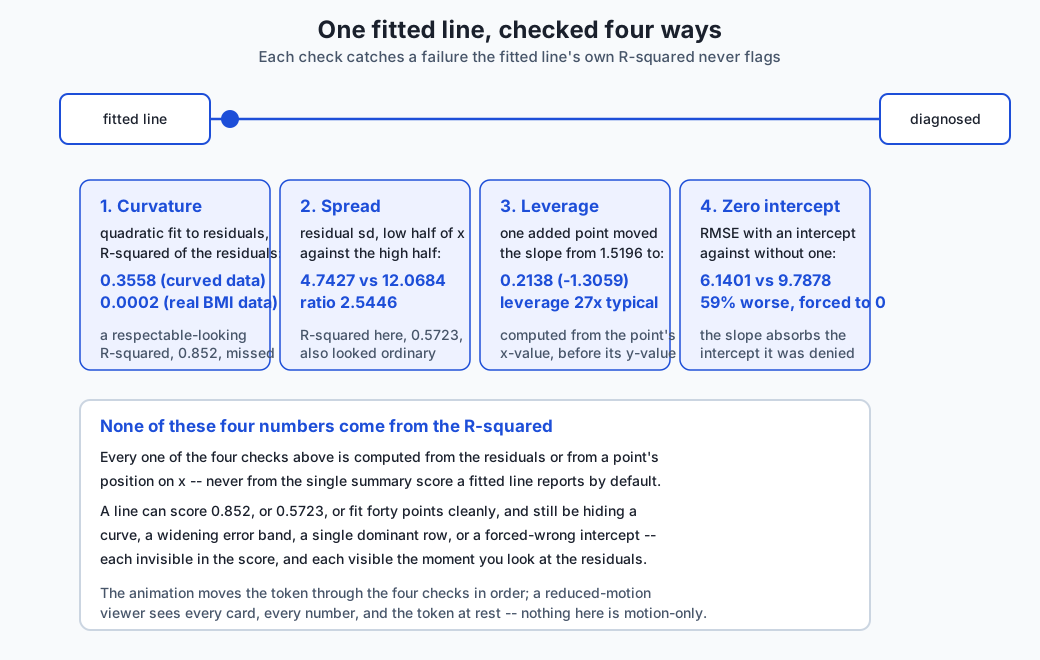
Positive, negative, negative, negative, positive. The line is too high at the edges and too low in the middle, in a pattern that repeats every single time this dataset is fit. That is not noise. That is the shape of a curve the line cannot draw, showing up exactly where the line refuses to bend. Fit a quadratic to those five numbers on their own and it explains 35.58 percent of the residuals’ own variance — more than a third of what the line filed away as “error” is actually structure the line was the wrong shape to capture.
The scatterplot did not show this clearly. The R-squared did not show it at all — 0.852 is what a genuinely good linear fit looks like too. The only place this failure is visible is a plot of the residuals against x, and today’s lab builds that plot as five printed numbers because a moving picture is not required to see a U-shape in five numbers that go up, down, down, down, up.
This is the day the line stops being a picture and starts being an object you can interrogate. A fitted line is three numbers — a slope, an intercept, and how much of the target’s spread it accounts for — plus a promise, four assumptions, about the data it was fitted to. Every one of those four assumptions can fail silently, in a way the line itself will never tell you about. This lesson measures what each failure looks like, on purpose, so you know the shape to look for when it happens by accident.
The idea in plain language
A straight line is a rule for turning one number into another: multiply
by a slope, add an intercept. y = slope * x + intercept. That is the
entire model. No hidden state, no branching, no memory of any row it has
not seen. Every prediction the model will ever make comes from those two
numbers and whatever x you hand it.
Fitting the line means choosing the slope and intercept that make the
model’s predictions come as close as possible, on average, to the actual
y-values in the data you have. “As close as possible” needs a precise
definition — Day 149 owns that definition and the reasons squared error
is the usual choice — but for today, trust scikit-learn’s
LinearRegression to find the best slope and intercept for whatever data
you give it, the same way Day 146 trusted fit to do the right thing
without asking you to write the arithmetic yourself.
Once it is fitted, the line makes a specific, falsifiable claim about the world: that the relationship between x and y is a straight one, that the scatter around that line is roughly the same width everywhere, that one observation is not silently steering the whole line, and that the leftover noise looks like noise rather than like a second signal. Four claims. Today’s lab breaks each one on purpose and measures exactly what the breakage looks like, so that when you meet a broken one by accident in real data, you recognize the shape.
Here is the everyday version, briefly, before the analogy gets its own section later: think of the line as a rule of thumb someone gives you — “every extra ten years of experience is worth about eight thousand a year in salary.” That rule of thumb is only as good as the situations it was built from. It can be a genuinely useful summary and still be the wrong shape (maybe the real relationship levels off after twenty years), built on unevenly reliable data (maybe salaries get noisier at senior levels), vulnerable to one extreme case (one enormous outlier salary can drag the whole rule toward it), and stated with more confidence than it deserves if nobody ever attaches a margin of error to it.
Historical background
The method behind today’s fitted line is older than the phrase “machine learning” by about two centuries.
Adrien-Marie Legendre published the method of least squares in 1805, in an appendix to a book on computing the orbits of comets — a practical problem of reconciling many imperfect astronomical observations into one best estimate. Carl Friedrich Gauss published his own account of the method in 1809, in Theoria Motus Corporum Coelestium, and claimed to have been using it since 1795. The resulting priority dispute between the two is one of the best-documented disagreements in the history of statistics, and it is generally accepted today that they arrived at the same idea independently: minimize the sum of squared errors between a model’s predictions and the observed data.
The word “regression” itself arrived later and from an entirely different direction. Francis Galton, studying the heights of parents and their adult children in the 1880s, noticed that tall parents tended to have children who were tall, but on average a little shorter than themselves — and that short parents’ children tended to be a little taller than their parents. He called this “regression towards mediocrity” in an 1886 paper, and the name for the phenomenon became the name for the technique used to study it, even though most uses of linear regression today have nothing to do with any tendency to average out. Galton’s protégé Karl Pearson formalized the correlation coefficient in the 1890s, giving the field the other half of the vocabulary this lesson uses: R-squared is, for a simple linear regression, exactly the square of Pearson’s correlation coefficient between x and y.
What has changed since 1805 is not the arithmetic — the normal equations
Legendre and Gauss derived are, up to notation, exactly what
LinearRegression.fit solves today — but the scale and the automation.
Where Legendre solved a handful of equations by hand for a handful of
comet observations, scikit-learn solves the same equations for datasets
of any size, instantly, and the discipline that has grown up around
checking the fit — residual plots, leverage, the four assumptions this
lesson measures — is largely a twentieth-century development, once
computers made it practical to check a fit’s assumptions as routinely as
computing the fit itself.
What it is — and what it is not
Simple linear regression is a model with exactly two learned numbers: a slope and an intercept, fitted to one predictor and one target. “Simple” here is a technical term, not a value judgment — it means one predictor, as opposed to “multiple” linear regression’s several predictors, which Day 150 owns. Today’s lab uses BMI, and only BMI, to predict a one-year diabetes-progression score.
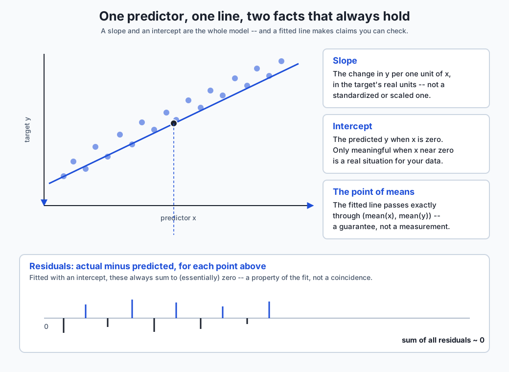
Two facts about a fitted simple linear regression with an intercept are true always, on any dataset, for a reason that has nothing to do with today’s particular numbers:
The fitted line passes exactly through the point (mean of x, mean of y). Today’s lab measures this to eight decimal places on the diabetes
data: the model’s prediction at the mean BMI is 152.1335, and the mean of
the actual target is also 152.1335. Not close. Equal, to within floating
point.
The residuals sum to (essentially) zero. Add up every leftover error
across all 442 rows and the total is -1.67e-11 — zero, for any practical
purpose, and it would be exactly zero under exact arithmetic. This is not
a lucky property of BMI and diabetes progression. It follows from how
least squares finds its solution, which Day 149 derives properly; today
you can rely on it and check it, the way Day 144 relied on and checked
that a validation set’s optimism is a computable quantity rather than
taking either fact on faith.
Now what a fitted line is not.
It is not evidence of causation. A slope of 10.2331 says that, in this dataset, higher BMI and higher disease-progression scores moved together by about that much on average. It says nothing about whether changing someone’s BMI would change their score by that amount, or whether some third factor drives both. Day 119 covered this distinction properly; today’s lesson does not re-argue it, but the coefficient you are about to read is exactly the kind of number people over-interpret this way, so it is worth restating plainly: a regression coefficient is a statement about association in the data you fitted, not a lever you can pull in the world.
A high R-squared is not evidence the model is correctly shaped. This lesson’s opening measurement — 0.852 on data with a real, substantial curve the line cannot draw — is the whole argument for this sentence. R-squared answers “how much of the target’s variance does this line explain,” and a curve can explain plenty of variance while still being systematically wrong in a way that matters.
The standard error of a coefficient is not a statement about how “big” the effect is. It is a statement about how precisely the effect was measured, given the sample the model saw. A slope of 10.2331 with a standard error of 0.6738 is a precisely measured moderate effect; a slope of 200 measured on four rows with a standard error of 150 is an imprecisely measured number that happens to look large.
Why it was created and what problems it solves
The problem simple linear regression solves is narrow and specific: summarize the relationship between one number and another with the smallest possible model that still says something quantitative.
Before you have any model, “BMI and disease progression seem related” is a qualitative claim you could support with a scatterplot and a shrug. After fitting a line, you have a number: 10.2331 points of progression per unit of BMI, with a standard error of 0.6738, which converts the shrug into a claim you can state precisely, defend with a confidence interval, and — crucially — check.
A slope with no standard error is barely more useful than the shrug it
replaced, because you cannot tell whether it reflects a real, reliably
measured relationship or noise that happened to organize itself into a
line. This lesson’s BMI slope divided by its own standard error is
10.2331 / 0.6738 = 15.19 — the slope is about fifteen standard errors
away from zero, which is the kind of number that lets you say, with real
confidence, that this is not noise. Contrast that with a coefficient two
standard errors from zero, which is the conventional (if somewhat
arbitrary) line past which people start calling a result “significant” —
fifteen is not a borderline case in either direction.
The four assumptions this lesson measures each solve a distinct failure mode that a naive “just fit a line and read the slope” approach walks straight into.
Linearity solves the problem of describing a relationship with the wrong shape entirely. Section “How it works” measures what happens when you skip this check: a good R-squared, a completely wrong picture of how x and y actually relate.
Constant variance (homoscedasticity) solves the problem of a model whose confidence should not be uniform but is reported as if it were. When the spread of the noise around the line grows with x, a single standard error computed across the whole dataset understates your uncertainty at high x and overstates it at low x — the model does not know this about itself, and neither will you unless you check.
No dominant point solves the problem of a fit that is really a report on one row. Section “How it works” measures a single added point cutting a slope by more than 85 percent, out of forty-one total rows. Nothing about the R-squared or the fitted equation flags which points did the work.
Roughly normal residuals solves the problem of a standard error that assumes a shape the data does not have. The formula this lesson uses for the slope’s standard error, and the confidence interval built from it, both assume the noise is reasonably well-behaved (in the everyday sense — symmetric, no wild extreme values dominating). A heavily skewed or heavy-tailed residual distribution can make that interval too narrow or too wide, silently.
How it works
Fitting the line, and the two facts that always hold
LinearRegression().fit(X, y) finds the slope and intercept that
minimize the sum of squared residuals — Day 149 derives why squared error
specifically, and Day 153 rebuilds the fit from first principles. Today,
treat the fit as a black box that returns two numbers, and check what
those two numbers actually mean.
On BMI (in its raw, unscaled units — more on that in a moment) predicting one-year disease progression, across all 442 rows of the classic diabetes dataset:
  slope      : 10.2331
  intercept  : -117.7734
  R-squared  : 0.3439
Read the slope as a sentence: each additional unit of BMI is associated
with about ten more points of one-year disease progression, on this
population. That sentence is only writable because the BMI column is in
real units — kilograms per square meter, roughly 18 to 42 across this
dataset — rather than the mean-centred, unit-norm-scaled version
load_diabetes() returns by default. Call it with scaled=False and
every column keeps its original units; skip that argument and the slope
is a number with no sentence attached to it, because “one more standardized
unit of BMI” is not a quantity anyone experiences.
The intercept, -117.7734, is what the model would predict at BMI = 0 —
a BMI of zero is not a real situation, so the intercept here is not
independently meaningful; it exists to make the line pass through the
data correctly, not to be read on its own. This is common and not a
defect: an intercept only carries its own sentence when x = 0 is a
realistic case.
R-squared, 0.3439, says BMI alone accounts for about a third of the variance in the progression score — a real, moderate, single-predictor relationship, and a reminder that most of the variation in this outcome is explained by something other than BMI, which is exactly what you would expect from one predictor among the several (age, blood pressure, several blood-serum measurements) the fuller dataset provides and Day 150 will use together.
Both structural facts hold, measured directly rather than assumed:
  predicted value at mean BMI : 152.1335
  mean of the target           : 152.1335
  difference                   : 0.00e+00

  sum of the 442 residuals     : -1.67e-11
The slope has a standard error, and it is worth computing
A slope fitted on 442 rows would come out at least slightly different on a fresh sample of 442 rows from the same population. The standard error quantifies how different, using the same arithmetic Days 117-118 and Day 144 both used for a sampling proportion, applied here to a slope:
SE(slope) = s / sqrt(sum((x - mean(x))^2))where s^2 is the residual variance with the two degrees of freedom
spent fitting the slope and intercept subtracted off. On the BMI model:
  slope standard error : 0.6738
  95% confidence interval : [8.9125, 11.5538]
  slope / standard error  : 15.19
A 95 percent interval from 8.91 to 11.55 says: if you drew many fresh 442-row samples from the same population and fitted a line to each, about 95 percent of the resulting slopes would fall in that range. It does not mean there is a 95 percent chance the true slope is in that specific interval — a common and understandable misreading — but for practical purposes it tells you the plausible range of effect sizes given what you measured, which is usually what you actually wanted to know.
Recovering a slope you know to be true
The BMI model’s slope is measured against real data with an unknown true relationship. To see the standard-error logic from the other direction — watching an estimate converge on a number you fixed yourself — construct data with a known true slope of 5.0, fit a line, and measure how far the estimate lands from 5.0 as the sample size grows:
       n   mean abs error
      20   0.2315
      50   0.1556
     200   0.0780
    1000   0.0357
    5000   0.0159
Averaged over 200 independently generated datasets at each size — one
draw is an anecdote, and Day 144 made exactly this point about a single
seed. The error shrinks steadily, and it shrinks at roughly the rate the
standard-error formula predicts: quadrupling the sample size should
roughly halve the error, because the error scales like one over the
square root of n. From n=20 to n=200 (ten times the rows) the measured
ratio is 0.3369, close to the predicted 1/sqrt(10) = 0.3162; from n=20
to n=5000 (250 times the rows) the ratio is 0.0687 against a predicted
1/sqrt(250) = 0.0632. Close, not exact — this is itself a measured
quantity with its own sampling noise, which is why the lab asserts a
range rather than a single figure.
Two ways a fit can look fine and be wrong
Both of the following construct data where the R-squared alone gives no warning, and only a residual plot exposes the problem.
Curvature. Data generated from y = 2.0 + 0.5 * x^2 + noise, fitted
with a straight line, scored an R-squared of 0.852 — the opening
measurement of this lesson. The residuals, binned by x, trace the missed
curve exactly:
     x     mean residual
  0.96        +4.2216
  2.85        -1.9594
  4.84        -3.6829
  6.97        -2.3803
  8.92        +3.8010
To turn “the residuals look U-shaped” into a number rather than an impression, fit a quadratic curve to the residuals themselves (as a diagnostic — not a second model of the data) and see how much of the residuals’ own variance it explains:
  quadratic fit to the residuals, R-squared : 0.3558
  correlation of residuals with x-squared   : 0.1480
Over a third of what the line called “error” is missed structure. Compare
this against the same diagnostic run on the real BMI model’s residuals —
where there is no known missed curve — and it comes back at 0.0002,
essentially zero. That contrast, not either number in isolation, is how
you tell “there is a real missed curve” from “this is just noise”:
compute the same diagnostic on data you trust is linear, see what a clean
number looks like, and compare.
Heteroscedasticity. Data generated so the noise around the line grows
with x — noise_sd = 0.8 * x — fitted with a straight line, scored an
R-squared of 0.5723, also entirely unremarkable. But split the residuals
at the median of x and compare their spread:
  residual sd, low half of x  : 4.7427
  residual sd, high half of x : 12.0684
  ratio                        : 2.5446
The scatter around the fitted line is two and a half times wider at high x than at low x. The fitted line itself stays roughly correct on average — least squares does not become biased just because the noise has unequal spread — but any confidence interval built from a single, dataset-wide standard error is wrong everywhere except right at the average spread, understating your uncertainty at high x and overstating it at low x. A residual plot with x on the horizontal axis and residuals on the vertical shows this as a widening fan; a scatterplot of the raw data shows something that, at a glance, looks like ordinary noisy data.
One point that moves the whole line
Forty ordinary points, a clean linear relationship, fitted:
slope, forty ordinary points : 1.5196Add one point, at x = 40 (four times beyond the range of the other forty, which sit between 0 and 10) with a y-value that ignores the trend entirely, and refit:
  slope, plus one point at x=40, y=5 : 0.2138
  change                              : -1.3059
One row, out of forty-one, cuts the slope by more than 85 percent. The mechanism has a name — leverage — and a formula that depends only on the point’s position on the x-axis, computed before its y-value even enters the picture:
leverage = 1/n + (x - mean(x))^2 / sum((x - mean(x))^2)For the added point: 0.8048. For the average of the other forty:
0.0299. A ratio of nearly 27 — the added point has almost twenty-seven
times the pull of an ordinary one, purely because of where it sits on the
x-axis. A point can have high leverage and cause no trouble at all, if
its y-value happens to agree with the trend the other points already
established; leverage measures the potential to move the fit, and
whether that potential gets used depends on the y-value too. Here it very
much was.
fit_intercept=False, and what it costs
scikit-learn’s LinearRegression fits an intercept by default, and the
fit_intercept=False option forces the line through the origin. On data
whose true intercept is 25.0 and whose x-values never come near zero (they
range from 5 to 25):
  RMSE, fit_intercept=True  : 6.1401
  RMSE, fit_intercept=False : 9.7878
  ratio                     : 1.5941
Forcing the intercept to zero makes the error nearly 60 percent worse,
and the reported slope changes to compensate: 4.4232 against a true
slope of 3.0. The model has no way to represent “the line does not pass
through the origin” except by tilting, so it tilts, and the resulting
slope is not a fair estimate of the real relationship — it is
contaminated by the intercept the model was not allowed to fit.
fit_intercept=False is occasionally the right choice — some physical
quantities genuinely must be zero at x = 0 — but it is a strong,
checkable claim about the data, not a default worth reaching for
casually.
An everyday analogy
A tailor’s rule of thumb: “add one inch of sleeve length for every two inches of height above five foot six.”
That rule is a simple linear regression someone fitted, informally, from years of measuring customers. It has a slope (half an inch of sleeve per inch of height) and an implicit intercept (the sleeve length at five foot six). It is useful precisely because it compresses a lot of individual measurements into two numbers a tailor can carry around in their head.
The slope and intercept are real quantities, in real units — the tailor is not saying “half a standardized unit,” they are saying half an inch, the way this lesson insisted on raw BMI units rather than scaled ones.
The rule assumes the relationship is a straight line across the whole range it is applied to. For most adult customers that is probably fine. Apply it to a child, far outside the range of adults the rule was built from, and it likely breaks down — the true relationship between height and sleeve length is not straight all the way down to zero, the same way this lesson’s curved dataset was not straight at all despite the line’s 0.852 R-squared. A tailor who has only ever measured adults has no way to know this from their own experience; they would need to go measure some children specifically to find out, the way this lesson had to compute the quadratic-fit diagnostic to find the curve the eye and the R-squared both missed.
The rule assumes the tailor’s measuring error is about the same size for a short customer and a tall one. If taller customers are harder to measure precisely — looser clothing, more variation in posture — the rule’s real precision is worse at the tall end than the short end, in exactly the shape this lesson’s heteroscedasticity section measured: a fitted line that looks fine on average while its honest uncertainty fans out.
One extraordinarily tall customer, measured once, could shift the tailor’s rule of thumb far more than any ordinary customer would, purely because that customer sits so far outside the usual range — this lesson’s leverage point, in cloth. If that one measurement happened to be recorded wrong, the whole rule would tilt to accommodate a mistake, the same way one bad row cut today’s measured slope by more than 85 percent.
And forcing the rule through the origin — insisting sleeve length must
be exactly zero at zero height — would be absurd for a tailor and is
exactly as absurd, mathematically, as fit_intercept=False on data whose
x-values never approach zero. The tailor’s rule works because it is
allowed an intercept; so does today’s BMI model.
Examples in practice
Fitting and reading a coefficient
from sklearn.datasets import load_diabetes
from sklearn.linear_model import LinearRegression

data = load_diabetes(scaled=False)
bmi = data.data[:, 2].reshape(-1, 1)
y = data.target

model = LinearRegression().fit(bmi, y)
print(model.coef_[0], model.intercept_, model.score(bmi, y))
scaled=False is the entire trick, and it is easy to miss: the default
call to load_diabetes() returns every column already mean-centred and
scaled to unit norm, which is convenient for some modelling tasks and
useless for reading a coefficient in real units. This is the same kind of
silent trap Day 144 documented for train_test_split not stratifying by
default — the tool’s default is a choice, not a neutral starting point,
and today’s is scaled=True, the wrong one for interpretation.
Reading a residual plot by hand
You do not need a plotting library to catch curvature or fanning; binning the residuals by x and printing the group means, as this lesson did throughout, is the same diagnostic with numbers instead of pixels:
import numpy as np

order = np.argsort(x.flatten())
x_sorted, resid_sorted = x.flatten()[order], residuals[order]
for group in np.array_split(np.arange(len(x_sorted)), 5):
    print(round(x_sorted[group].mean(), 2), round(resid_sorted[group].mean(), 4))
Five numbers that go up, down, down, down, up are exactly as diagnostic as a scatter of a thousand points forming a visible U — the shape is what matters, and a shape can be read from a table.
A salary study with a leverage problem
An analyst regresses salary on years of experience across a team of
twenty engineers, gets a clean-looking fit, and reports it to leadership.
One engineer on the team is the founder, with thirty years of experience
and a salary set by equity negotiations that have nothing to do with the
usual experience curve. That single row, sitting far outside the range of
the other nineteen, can dominate the fitted slope the way today’s added
point at x = 40 dominated a forty-point dataset — and the report would
describe the founder’s outlier salary as if it were evidence about how
experience and pay relate for everyone else on the team. Checking leverage
before publishing the coefficient — which rows have unusually large
(x - mean(x))^2 — is a five-minute check that would have caught this.
A residual plot that would have caught Anscombe’s quartet
Statistician Francis Anscombe constructed four small datasets in 1973, each producing nearly identical summary statistics — same mean, same variance, same correlation, same fitted regression line — while looking completely different when plotted. One is a clean linear relationship. One is a clear curve fitted with a straight line. One has a single outlier driving the whole fit. One is nearly a vertical line of identical x-values with one point determining the slope entirely. All four would report the same R-squared; only a residual plot (or, per this lesson, the same diagnostics run without a plot) tells them apart. It remains one of the clearest illustrations available of exactly the point this lesson measures: summary statistics can agree completely while the underlying relationship does not.
Implications: security, privacy, performance, scalability, and cost
The cost of trusting R-squared alone is entirely a cost of finding out late. A model deployed on the strength of a 0.852 R-squared, with nobody having looked at the residuals, will make systematically wrong predictions at both ends of its input range — underestimating at the extremes, overestimating in the middle, or the reverse — and nothing in its own reported metric will have warned anyone. The check that would have caught it is five printed numbers.
Leverage is a data-quality and, at scale, a data-integrity concern. A single erroneous or adversarially placed row far outside the normal range of a predictor can move a fitted model’s coefficients far more than its single-row weight in the dataset would suggest — this lesson measured almost twenty-seven times the pull of an ordinary point. In a pipeline that retrains automatically on incoming data, an unusual input is not just a modelling nuisance; it is an integrity question, and the leverage formula gives you a way to flag candidate rows for review before they reach the fit, independent of whether their label looks reasonable.
Fitting a simple linear regression is computationally trivial and stays that way at scale. The normal equations for one predictor are a closed form — no iteration, no convergence warnings, and fitting the entire 442-row diabetes dataset or a synthetic dataset of several thousand rows both complete in a small fraction of a second on ordinary hardware, with no GPU involved at any point in this lesson or its lab.
Interpretability is itself a cost-saving property, not just a nicety. A one-predictor linear model that says “ten points of progression per unit of BMI, standard error 0.67” can be checked, argued with, and explained to a non-technical stakeholder in one sentence. That is genuinely valuable in regulated or high-stakes settings, and it is a property this lesson’s model has and a more complex one might not — worth weighing against whatever accuracy a more complex model buys you, not assumed away.
Reporting a coefficient without its standard error is a form of
overstating precision, and overstated precision has a cost whenever a
decision gets made on the strength of a number that looked more certain
than it was. 10.2331 alone invites someone to treat that as exact.
10.2331 ± 0.6738 invites the correct question: is the range this
implies still meaningful for the decision at hand?
Alternatives: free, open source, and commercial
scikit-learn’s LinearRegression — used here
When to choose it: the default choice for ordinary least squares on any dataset that fits in memory. Free, BSD-3-Clause licensed, no paid tier. Every measurement in this lesson uses it.
How to use it: LinearRegression().fit(X, y), where X is a 2-D
array even for one predictor — bmi.reshape(-1, 1), not the flat array —
and y is a 1-D array of targets. model.coef_ and model.intercept_
hold the fitted parameters after fit returns.
Watch for: it does not compute a standard error, a confidence
interval, or a p-value for you — those come from statsmodels (below) or
from the manual formula this lesson used directly. LinearRegression
gives you the fit; the uncertainty is a separate, deliberate step.
statsmodels — described, and the honest note
When to choose it: when you want p-values, confidence intervals and a full regression summary table without computing the standard-error formula by hand, or when you are doing applied statistics work where that table is the expected output.
How to use it: statsmodels.api.OLS(y, statsmodels.api.add_constant(x)).fit()
returns a results object with a .summary() that prints coefficients,
standard errors, t-statistics, p-values and confidence intervals in one
table — everything this lesson computed by hand from the residuals, in
one call.
Honest note: statsmodels is not installed in this course’s
environment (see the shared authoring brief), and no output from it is
reproduced anywhere in this lesson or its lab. This description is drawn
from its public documentation, not from a run performed here.
Free versus paid: free and open source (BSD-3-Clause), no paid tier.
R’s lm() — described from documentation
When to choose it: the R programming language’s built-in linear
model function, lm(y ~ x), is the historical reference implementation
many statisticians learned regression on, and its summary() output —
coefficients, standard errors, R-squared, F-statistic — is close to a
direct ancestor of what statsmodels’ summary table now provides in
Python.
What it costs: R itself is free and open source. No output from it is reproduced here; this lesson and its lab are Python-only, and this description is for orientation if you encounter regression output from an R-based analysis elsewhere.
Excel’s Trendline and LINEST — described, and the honest note
When to choose them: a genuinely reasonable choice for a quick,
one-off linear fit on data already sitting in a spreadsheet, particularly
for a non-technical audience who will read the output directly in Excel.
LINEST additionally returns a standard error for the slope, in the same
spirit as this lesson’s exercise 1b.
What it costs: included with any Excel licence (Microsoft 365 subscription or a one-time purchase); free spreadsheet tools (LibreOffice Calc, Google Sheets) offer equivalent trendline and slope-fitting functions at no cost. No output from Excel is reproduced here.
Comparison with related concepts
| Concept | What it does | How it relates |
|---|---|---|
| Simple linear regression | one predictor, a straight line | Today’s subject: the geometry, the coefficient, the four assumptions |
| Multiple linear regression | several predictors, one linear combination | Day 150 — the design matrix, and what changes when predictors correlate with each other |
| Polynomial regression | a curve, fitted as a linear model in transformed features | Day 150 — the fix for exactly the curvature this lesson’s section 3 measured |
| Ridge and lasso regression | linear regression with a penalty on the coefficients | Day 151 — a different fix for a different failure: coefficients that are unstable, not wrongly shaped |
| Ordinary least squares | the specific fitting criterion LinearRegression uses | Day 149 — why squared error, not this lesson’s subject |
| Logistic regression | a linear model for a classification target, via a link function | Day 146’s estimator API, extended to a different kind of target |
| Correlation coefficient | a single number summarizing linear association, no fitted line | R-squared, for one predictor, is exactly the correlation coefficient squared |
| Robust regression (Huber, RANSAC) | fitting resistant to leverage points and outliers | The described-not-run extension for section “one point that moves the whole line” |
Two rows deserve a closing note.
R-squared and the correlation coefficient are the same information, restated. For simple linear regression specifically, R-squared is Pearson’s correlation coefficient, squared. Knowing this is worth more than it sounds: it means R-squared cannot exceed what the raw correlation between x and y already told you, and a low R-squared is not something a fancier fitting algorithm can fix if the true relationship with that one predictor is genuinely weak.
Polynomial regression is still linear regression, in the sense that
matters to the fitting algorithm — it fits a straight-line relationship
between the target and a set of features that happen to include x^2,
x^3, and so on. The model is a curve in x but a straight line (a linear
combination of features) in the transformed feature space. Day 150 covers
this properly; today’s lesson only needed the concept to name what it
diagnosed in the curvature section.
When to use it — and when not to
Use it as the first model you fit for any one-predictor numeric relationship, not because it is always the best model but because it is fast, fully interpretable, and gives you a baseline every fancier model should have to beat. If a random forest cannot outperform a one-line linear fit by a meaningful margin, that is worth knowing before you ship the random forest.
Always check the four assumptions before trusting the coefficient. Bin the residuals and look for curvature. Split them by x and compare spread. Compute leverage for any point that looks unusual on x alone. Check the residuals’ skewness for anything wildly asymmetric. None of these checks are expensive, and each one catches a specific, common way this lesson demonstrated a fit can look fine and be wrong.
Do not use a plain linear fit when the true relationship is known or suspected to be curved, without either transforming the predictor (Day 150) or choosing a different model entirely. This lesson’s 0.852 R-squared on genuinely quadratic data is the standing warning: a respectable score is not permission to skip the residual check.
Do not force fit_intercept=False unless x = 0 is a real, meaningful
situation in your data and you have a specific reason (often a physical
law) to believe the true relationship passes through the origin. This
lesson measured a 59 percent RMSE increase from getting this wrong.
Do not report a coefficient without its standard error, when the audience for that coefficient might make a decision based on how large or reliable it looks. “Ten points per unit of BMI” and “ten points per unit of BMI, give or take about two-thirds of a point, based on 442 observations” are different claims, and only the second one lets someone else judge whether the precision is good enough for what they need it for.
When you do not need it: when the relationship you care about involves more than one predictor from the start (go straight to Day 150’s multiple regression rather than fitting several single-predictor models and trying to combine them by hand), or when the target is categorical rather than continuous (logistic regression, or a classifier, is the right family — Days 141-147 already covered that setting).
The AI thread
The four assumptions this lesson measured are not specific to a two-parameter line — they are the first, smallest instance of questions every larger model faces in a harder-to-see form.
Curvature becomes “is the model the wrong shape for the relationship,” at any scale. A linear model that misses a curve produces a visible, checkable U-shape in its residuals, five printed numbers wide. A neural network with millions of parameters can miss structure in a subtler way — systematically wrong on a subgroup of its inputs — and the same discipline applies even though the check is harder to run: look at where the errors concentrate, not just at the aggregate score, the same way this lesson insisted on the residual plot over the R-squared alone.
Leverage becomes “which training examples had outsized influence on this model,” and the stakes go up with the model’s size. A single unusual row moved today’s forty-point slope by more than 85 percent. A large model trained on a scraped or crowd-sourced dataset can be similarly, if less visibly, shaped by a small number of unusual or mislabelled examples — and unlike today’s forty-point toy dataset, nobody can eyeball a training set of a billion rows to spot the equivalent of the point sitting at x = 40. Influence-function methods and data-attribution research exist specifically to answer, at scale, the question this lesson’s leverage formula answers by hand: which training examples pulled the fit the hardest.
Reporting an estimate without its uncertainty is exactly as tempting, and exactly as costly, when the estimate comes from a much larger model. A benchmark score, a win rate against a baseline, a preference judgment from an LLM evaluator — all of these are estimates with sampling noise the way today’s slope has a standard error, and the discipline this lesson practiced on two coefficients — attach the uncertainty, check whether the effect is actually distinguishable from nothing — is the same discipline a rigorous evaluation of any AI system needs, at any scale. The arithmetic gets harder as the model gets bigger. The obligation to do it does not go away.
Knowledge check
- A line fitted to 300 points scores an R-squared of 0.852. What additional check would tell you whether that number can be trusted as evidence the relationship is genuinely linear, and what did that check reveal in this lesson?
- Why does
load_diabetes(scaled=False)matter for interpreting a fitted slope, and what happens to the sentence “one more unit of X is associated with N more units of Y” if you skip it? - State the two facts that are true of any least-squares line fitted with an intercept, on any dataset. Are they measurements or guarantees, and how can you tell the difference?
- The BMI model’s slope is 10.2331 with a standard error of 0.6738. Explain what the resulting 95% confidence interval does and does not tell you.
- A dataset’s residuals have standard deviation 4.7427 in the low half of x and 12.0684 in the high half, while the fitted line’s R-squared looks ordinary. Name the assumption this violates and explain why the R-squared did not catch it.
- One added point, out of forty-one total, cuts a fitted slope by more than 85 percent. What single number, computed from that point’s x-value alone, would have flagged it as a candidate for scrutiny before its y-value was even considered?
fit_intercept=Falseon data whose x-values range from 5 to 25 and whose true intercept is 25 makes the RMSE about 59 percent worse. Why does forcing the intercept to zero also bias the fitted slope, rather than just leaving it wrong in a way that does not affect the slope?- A quadratic fit to a set of residuals explains 0.0002 of their variance in one case and 0.3558 in another. What does this diagnostic tell you that the original model’s R-squared does not?
Hands-on exercise
Today’s lab, One Line, Measured, fits exactly one predictor against one
target and then measures four specific ways that fit can mislead you even
while its R-squared looks fine.
Twelve exercises. The first three fit the BMI model, attach a standard error to its slope, and confirm the two facts that hold on any least-squares line with an intercept. The next two watch a known slope get recovered as the sample size grows. The next four measure curvature and heteroscedasticity — two ways a fit can look fine and be wrong — and two more measure a single high-leverage point and the cost of forcing the intercept to zero. The last contrasts the curvature diagnostic on data with a real missed curve against the same diagnostic on data that is genuinely linear.
Build the environment, then work through
starter/test_regression_claims.py, replacing one pytest.skip at a
time.
Expected output
The harness ends with:
---------------------------------------------------------------
14 checks, 0 failure(s)
and exits 0. pytest examples -q reports 16 passed, and
pytest starter -q reports 4 passed, 12 skipped until you begin.
The measured table includes:
  slope     : 10.2331  (points of progression per unit of BMI)
  intercept : -117.7734
  R-squared : 0.3439
  slope SE  : 0.6738   95% CI [8.9125, 11.5538]   t = 15.19
  quadratic fit to the residuals, R-squared : 0.3558   (on curved data)
  leverage of the added point : 0.8048   mean leverage of the other 40 : 0.0299
Validate your work
bash tests/run_tests.sh; echo "exit=$?"reports14 checks, 0 failure(s)andexit=0. Capture the harness’s own exit status..venv/bin/pytest examples -qreports16 passed..venv/bin/python3 examples/report_measurements.py | diff - expected-output/measured-values.txtproduces no output.- When you have finished every exercise,
pytest starter -qreports16 passed. - Break one assertion on purpose, confirm the harness fails, restore it.
Troubleshooting
My BMI slope, intercept or R-squared do not match. Check that you
passed scaled=False to load_diabetes. The default returns every
column mean-centred and scaled to unit norm — a completely different,
uninterpretable scale.
My slope-recovery numbers (exercise 2) differ slightly. Read
expected-output/FIELDS.md first. That table is an average over 200
seeded draws, and NumPy’s own documentation says its random generator
gives no stream-compatibility guarantee across versions. What must hold
on any version: the error strictly decreases as n grows.
import file mismatch. You ran pytest examples starter together.
Run them separately.
My leverage numbers differ. They should not, on the pinned versions —
the leverage dataset and the added point are both fully deterministic.
Check you passed a 2-D array (x.reshape(-1, 1)) to fit_line, not a
flat one.
Common mistakes
Trusting R-squared without checking the residuals. The whole first half of this lesson is the argument against this habit: 0.852 on data with real, substantial curvature the line cannot represent.
Calling load_diabetes() without scaled=False and then trying to
read the resulting slope as if it were in real units. It is not, and the
sentence “one more unit of BMI” is not writable from the scaled version.
Treating the intercept as meaningful when x = 0 is not a real
situation. The BMI model’s intercept, -117.7734, exists to make the
line fit correctly; it is not a claim about anyone with a BMI of zero,
because nobody has a BMI of zero.
Reporting a coefficient with no standard error, especially when the audience will use it to make a decision. A number with no attached uncertainty invites more confidence than it has earned.
Practice assignment
Take a one-predictor relationship you already have, or care about, and audit it the way this lesson audited BMI against disease progression.
- Fit the line in real units, and write the slope as one sentence a non-technical reader could act on: “one more [unit of X] is associated with [N] more [units of Y].” If you cannot write that sentence, the units are wrong somewhere.
- Attach a standard error and a 95% interval to the slope, using the formula in “How it works,” and say plainly whether the effect is distinguishable from zero given how many rows you have.
- Bin the residuals by x into five groups and print the group means. If the pattern is not roughly flat around zero, describe the shape and what curve it suggests the true relationship has.
- Split the residuals at the median of x and compare their spread. If the ratio is well above 1, name the practical consequence: your confidence interval is wrong somewhere across the range of x, even though the point estimate is probably fine.
- Compute the leverage of your five most extreme x-values and check whether any of them also have unusual y-values. If one does, refit without it and report how much the slope moves.
The deliverable is the audit, not a better-looking R-squared.
Extension challenge
Pick one and measure it.
- A robust alternative. Fit
HuberRegressororRANSACRegressorfrom scikit-learn on today’s leverage-point dataset and measure whether it resists the outlier the way plainLinearRegressiondid not. - Confidence interval coverage. Simulate 500 datasets with a known true slope, compute a 95% confidence interval on each, and measure what fraction actually contain the true value. Compare it to 0.95 and explain any gap.
- How weak can the curvature get before you stop seeing it? Scale down the quadratic coefficient in the curved dataset toward zero and find, by trial, roughly where the binned residual means stop showing a clear shape. Report what that implies about spotting mild non-linearity by eye versus by the quadratic-fit diagnostic.
- Multiple leverage points at once. Add two or three high-leverage points at different positions instead of one, and measure whether their combined effect on the slope adds up or partly cancels.
- A second predictor, informally. Add an unrelated random column to the BMI data and refit with both columns (a preview of Day 150). Measure whether the BMI coefficient changes, and by how much, when a second, irrelevant predictor joins it.
Quiz
Q1. A line fitted to 300 points scores an R-squared of 0.852, and the data was actually generated from a quadratic relationship. What does the R-squared alone tell you about whether the line is the right shape for the data?
- Nothing reliable -- a good R-squared can coexist with a real, substantial missed curve, which only a residual plot reveals
- That the fit is definitely correct, since 0.852 is close to the maximum of 1.0
- That the relationship is at least 85.2 percent linear, with the rest being noise
- That a larger dataset would push the R-squared toward 1.0 and resolve the question
Show answer
Answer: A. Nothing reliable -- a good R-squared can coexist with a real, substantial missed curve, which only a residual plot reveals
R-squared measures how much of the target's variance the line explains, which a wrong-shaped line can still do plenty of. This lesson's curved dataset binned residual means -- +4.2216, -1.9594, -3.6829, -2.3803, +3.8010 -- trace the missed curve exactly, and a quadratic fitted to those residuals explains 35.58 percent of their own variance. R-squared has no notion of "85.2 percent linear"; it is a single number about explained variance, not a shape diagnostic, and more data would not change the fundamental mismatch between a straight line and a curved relationship.
Q2. Why does `load_diabetes(scaled=False)` matter for reading the fitted BMI slope of 10.2331, and what goes wrong if you call `load_diabetes()` without it?
- Nothing changes; scaled=False only affects how fast the model trains
- The default scaled=True version mean-centres and unit-norm-scales every column, so the resulting slope is on an uninterpretable scale and the sentence "one more unit of BMI" is no longer writable
- scaled=False removes rows with missing BMI values, which the scaled version keeps
- scaled=False is required for scikit-learn to accept the data at all; the scaled version raises an error
Show answer
Answer: B. The default scaled=True version mean-centres and unit-norm-scales every column, so the resulting slope is on an uninterpretable scale and the sentence "one more unit of BMI" is no longer writable
The default `load_diabetes()` returns columns already mean-centred and scaled to unit norm, which is a completely different, uninterpretable scale for reading a coefficient. With `scaled=False`, BMI stays in its real units (roughly 18 to 42), and the fitted slope of 10.2331 becomes a sentence a clinician could read: one more unit of BMI is associated with about ten more points of one-year disease progression. Neither version raises an error or drops rows; the only difference is units.
Q3. Two facts hold for the BMI model's fitted line: it predicts exactly 152.1335 at the mean BMI, which equals the mean of the target, and its 442 residuals sum to -1.67e-11. What kind of facts are these?
- Coincidences specific to the diabetes dataset, which would not hold on a different dataset
- Measurements that happened to come out close to exact this time, within normal sampling variation
- Guarantees that follow from how a least-squares line with an intercept is fitted -- true on any dataset, not measurements that could have come out otherwise
- Evidence that BMI is a strong predictor of disease progression
Show answer
Answer: C. Guarantees that follow from how a least-squares line with an intercept is fitted -- true on any dataset, not measurements that could have come out otherwise
Both facts are structural properties of the least-squares solution with an intercept, true on any dataset for a reason that has nothing to do with BMI or diabetes specifically -- Day 149 derives why. They are not measurements with sampling variation attached (the residual sum is not "close to zero," it is zero up to floating point), and they say nothing about whether BMI is a strong predictor -- that is what R-squared and the standard error address, separately.
Q4. One point added to a forty-point dataset, at x=40 (well beyond the other points' range of 0 to 10), cuts the fitted slope from 1.5196 to 0.2138. What number, computed from that point's x-value alone, would have flagged it as worth scrutiny before its y-value was even considered?
- Its residual, which measures how far its y-value falls from the fitted line
- The overall R-squared of the model with and without the point included
- The point's rank when all y-values are sorted from smallest to largest
- Its leverage, computed as 1/n plus the squared distance from mean(x) divided by the sum of squared distances from mean(x) across all points
Show answer
Answer: D. Its leverage, computed as 1/n plus the squared distance from mean(x) divided by the sum of squared distances from mean(x) across all points
Leverage is a function of x alone -- it does not involve y at all, which is exactly why it can be computed before a point's outcome is even known. The added point's leverage measured at 0.8048 against a mean of 0.0299 for the other forty, a ratio of nearly 27. A residual requires the fitted line and the point's y-value, so it cannot flag a point in advance; R-squared is a whole-model summary, not a per-point diagnostic; and sorting y-values says nothing about a point's position on x.
Q5. A fitted line has an R-squared of 0.5723, which looks unremarkable. Splitting its residuals at the median of x shows a standard deviation of 4.7427 in the low half against 12.0684 in the high half. What does this reveal, and why didn't the R-squared catch it?
- Heteroscedasticity -- error whose spread grows with x. R-squared summarizes overall explained variance and has no way to represent how that error is distributed across x
- The model is overfitting, and R-squared should have been lower to reflect that
- A coding error in the residual calculation, since spread should always be constant
- That the true relationship is not linear, the same failure as the curvature check
Show answer
Answer: A. Heteroscedasticity -- error whose spread grows with x. R-squared summarizes overall explained variance and has no way to represent how that error is distributed across x
Heteroscedasticity means the noise around the line is not equally wide everywhere -- here, the spread more than doubles from the low half of x to the high half, a ratio of 2.5446. The fitted line itself stays roughly unbiased; what breaks is any single, dataset-wide standard error, which understates uncertainty at high x and overstates it at low x. R-squared is a single aggregate number and has no mechanism to flag an uneven spread; this is a distinct failure from curvature, which is about the line's shape rather than the noise's spread.
Q6. `fit_intercept=False` is applied to data whose x-values range from 5 to 25 and whose true intercept is 25.0. RMSE gets about 59 percent worse, and the fitted slope changes from close to the true value of 3.0 to 4.4232. Why does forcing the intercept to zero also distort the slope, rather than leaving the slope correct and only the intercept wrong?
- It does not actually affect the slope; the 4.4232 figure is measurement noise
- The dataset's x-values being far from zero causes a numerical overflow that corrupts the slope
- fit_intercept=False also removes the R-squared calculation, so the slope reported is meaningless
- The model has no separate parameter left to represent "the line does not pass through the origin," so the slope tilts to compensate, and the resulting slope is a distorted estimate of the true relationship
Show answer
Answer: D. The model has no separate parameter left to represent "the line does not pass through the origin," so the slope tilts to compensate, and the resulting slope is a distorted estimate of the true relationship
With only one free parameter (the slope) and no intercept to absorb the true offset, the line is forced through the origin regardless of where the data actually sits, and the only way to reduce error given that constraint is for the slope to tilt -- which is exactly what happened, moving from close to the true 3.0 up to 4.4232. This is a real, measured effect, not noise; R-squared still computes normally; and there is no overflow involved, just a genuinely worse and biased fit.
Q7. A slope of 10.2331 has a standard error of 0.6738, giving a 95% confidence interval of [8.9125, 11.5538]. What does that interval actually tell you?
- That there is a 95% chance the true slope lies in exactly this interval
- That 95% of the individual data points fall within this range of the fitted line
- That if you drew many fresh samples of the same size from the same population and fitted a line to each, about 95% of the resulting slope estimates would fall in a range like this one
- That the model is 95% accurate at predicting new BMI values
Show answer
Answer: C. That if you drew many fresh samples of the same size from the same population and fitted a line to each, about 95% of the resulting slope estimates would fall in a range like this one
A confidence interval is a statement about the procedure's long-run behaviour across repeated sampling, not a probability statement about one fixed true value being in one fixed interval -- a common and understandable misreading, but a different claim. It says nothing about where 95% of the individual data points fall (that is a much wider range, since it is about y-values around the line, not about the slope estimate), and it makes no claim about prediction accuracy at all.
Q8. A quadratic fit to a set of residuals explains 0.0002 of their variance on the real BMI model and 0.3558 on a deliberately curved dataset. Why is the contrast between these two numbers more useful than either number alone?
- It is not more useful; only the largest number, 0.3558, matters for deciding whether a fit has a problem
- It proves that BMI data can never have curvature, unlike synthetic data
- It shows that the BMI model is a better fit than the curved-data model in every respect
- The contrast calibrates what "essentially zero" and "real structure" look like on this diagnostic, letting you judge a new dataset's number against a known-clean baseline and a known-broken one, rather than guessing at a threshold
Show answer
Answer: D. The contrast calibrates what "essentially zero" and "real structure" look like on this diagnostic, letting you judge a new dataset's number against a known-clean baseline and a known-broken one, rather than guessing at a threshold
Without a reference point, a lone number like "0.05" or "0.15" from this diagnostic on an unfamiliar dataset is hard to judge -- is it noise, or a real signal? Seeing 0.0002 on data known to be linear and 0.3558 on data known to have real curvature gives two calibration points to compare a new measurement against. It says nothing general about which model is "better" (they are testing different things) and nothing about whether BMI data specifically could ever show curvature -- only that this particular model, on this diagnostic, did not.
Glossary
- Simple linear regression
- A model with exactly two learned numbers -- a slope and an intercept -- fitted to one predictor and one target so their squared errors are as small as possible. "Simple" means one predictor, as opposed to multiple linear regression's several predictors.
- Slope
- The change in the predicted target per one unit of the predictor, in the target's real units. Measured here at 10.2331 points of disease progression per unit of BMI -- only interpretable in raw units, not the mean-centred, unit-norm-scaled default scikit-learn's diabetes dataset returns.
- Intercept
- The predicted target value when the predictor is zero. Only independently meaningful when a predictor value of zero is a realistic situation; otherwise it exists to make the line fit correctly rather than to be read on its own.
- Residual
- The leftover error at one row -- actual target value minus predicted value. Residuals are what a residual plot examines, and their pattern reveals what a single summary score like R-squared cannot.
- R-squared
- The proportion of the target's variance a fitted line explains, from 0 to 1. Measured at 0.3439 for BMI predicting disease progression, and at a respectable-looking 0.852 on data with real, substantial curvature the line was the wrong shape to capture -- the standing warning of this lesson.
- Standard error of a slope
- How much a fitted slope would wobble under a fresh sample of the same size, computed from the residual variance and the spread of the predictor. Measured at 0.6738 for the BMI slope, giving a 95% confidence interval of [8.9125, 11.5538].
- Point of means
- The point (mean of x, mean of y). A least-squares line fitted with an intercept passes through this point exactly, on any dataset -- a guarantee that follows from the fit, not a coincidence.
- Residual sum
- The total of all residuals across a dataset. Exactly zero, up to floating point, for any least-squares line fitted with an intercept -- measured at -1.67e-11 on 442 rows here.
- Linearity assumption
- The claim that the true relationship between predictor and target is a straight line. Broken by construction in this lesson's curved dataset, where an R-squared of 0.852 gave no warning and only the binned residual means -- +4.2216, -1.9594, -3.6829, -2.3803, +3.8010 -- revealed the missed curve.
- Homoscedasticity
- The assumption that the scatter of errors around the fitted line is roughly the same width everywhere. Its opposite, heteroscedasticity, was measured here as a residual standard deviation of 4.7427 in the low half of the predictor against 12.0684 in the high half.
- Leverage
- A measure of a point's potential to pull a fitted line toward itself, computed from its predictor value alone -- before its target value is even considered. Measured at 0.8048 for one added point against a mean of 0.0299 for forty ordinary points, a ratio of nearly 27.
- fit_intercept
- A `LinearRegression` argument that, when set to False, forces the fitted line through the origin. Measured to cost 59 percent worse RMSE and a biased slope on data whose true intercept was 25.0 and whose predictor values never approached zero.
- Quadratic-fit-to-residuals diagnostic
- Fitting a quadratic curve to a set of residuals (not to the original data) and reading how much of the residuals' own variance it explains. Near zero on genuinely linear data (0.0002, measured on the real BMI model) and substantial where curvature was missed (0.3558, measured on deliberately curved data).
- Skewness
- A rough measure of a distribution's asymmetry, zero for a perfectly symmetric one. Used here as an informal check on whether a model's residuals look roughly normal -- 0.156 for the BMI model's residuals, mildly asymmetric and not alarming.
- Correlation-causation distinction
- The principle, established on Day 119, that a regression coefficient describes association in the data it was fitted on and says nothing on its own about whether changing the predictor would change the target. A slope is not a lever.
- Anscombe's quartet
- Four datasets constructed by Francis Anscombe in 1973 that share nearly identical summary statistics -- including the same fitted regression line -- while looking completely different when plotted, an early and influential illustration of exactly this lesson's argument for residual plots.
- Method of least squares
- The fitting criterion `LinearRegression` uses: choose the slope and intercept that minimize the sum of squared residuals. Published by Legendre in 1805 and by Gauss in 1809, who claimed prior use from 1795; Day 149 derives why squared error specifically.
- Robust regression
- A family of fitting methods, such as scikit-learn's HuberRegressor and RANSACRegressor, designed to resist the influence of high-leverage points and outliers that an ordinary least-squares fit does not resist. Described here from documentation; not run in this lesson's lab.
Sources and further reading
- LinearRegression -- scikit-learn API reference — scikit-learn developers (accessed 2026-08-27)
- load_diabetes -- scikit-learn API reference, including the raw-versus-scaled distinction — scikit-learn developers (accessed 2026-08-27)
- Linear Models -- scikit-learn user guide — scikit-learn developers (accessed 2026-08-27)
- Simple linear regression — Wikipedia (accessed 2026-08-27)
- Leverage (statistics) — Wikipedia (accessed 2026-08-27)
- Anscombe's quartet -- four datasets with the same fitted line and wildly different residuals — Wikipedia (accessed 2026-08-27)
- Ordinary least squares — Wikipedia (accessed 2026-08-27)
- numpy.polyfit -- NumPy reference, used here as a residual diagnostic — NumPy developers (accessed 2026-08-27)
Kept in this browser, no account needed. Your progress page turns the whole record into one link you can bookmark or open on another device.