Machine Learning › Regression › Day 149
Day 149: Loss Functions and Least Squares

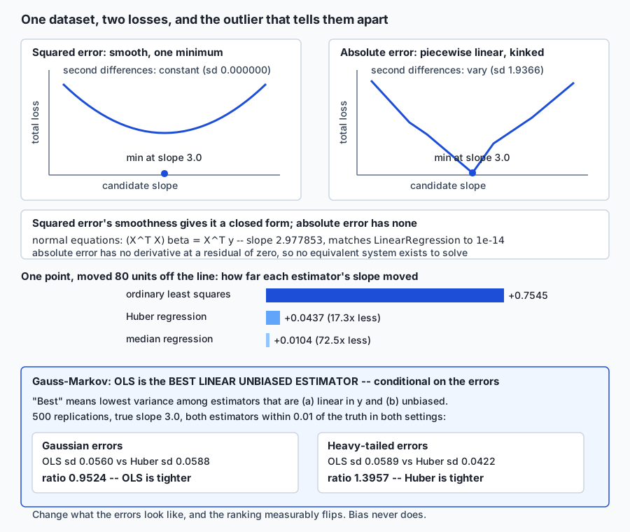
After this lesson you will have watched a single outlier, moved 80 units off an otherwise ordinary line, move a least-squares slope by 0.7545 while a Huber fit moves 0.0437 and a median fit moves 0.0104 -- seventeen and seventy-two times less -- on the exact same data. You will have confirmed by grid search, not by citation, that squared error is minimised by the mean and absolute error by the median, and that this single fact is the entire reason the two losses disagree about outliers. You will solve the normal equations directly and watch them match scikit-learn's LinearRegression to thirteen decimal places, and understand precisely why absolute error has no equivalent closed form. You will sweep Huber's delta parameter and watch it interpolate continuously between the two, landing exactly on the least-squares answer once the threshold grows large enough. And you will measure Gauss- Markov's theorem instead of reciting it: fit the same estimators five hundred times each under Gaussian errors and under heavy-tailed errors, and watch ordinary least squares win the precision contest in one setting and lose it in the other -- proof that "best linear unbiased estimator" is a conditional claim, not an unconditional one.
Hands-on lab for this lesson
Lab files on GitHub: https://github.com/ai-roadmap-365/ai-roadmap-365.github.io/tree/main/labs/sections/machine-learning/day-149-loss-functions-and-least-squares
- Get the hands-on files. Clone the labs repository once (you can reuse this clone for every lesson). This works on macOS, Linux, and Windows (PowerShell or WSL):
git clone https://github.com/ai-roadmap-365/ai-roadmap-365.github.io.git cd ai-roadmap-365.github.io - Open this lesson's lab. Move into the directory for this specific day. Every lab lives at the same predictable path — section / subsection / week / day:
cd labs/sections/machine-learning/day-149-loss-functions-and-least-squares - Read the lab guide. Open `README.md` in that directory. It lists the exact commands, what each does, the expected output, and how to check your work — read it before running anything.
- Run it and check your work. Follow the README's "How to run" section: run the example first to see the finished result, then complete the numbered exercises in `starter/`, then run the tests. The tests pass (exit 0) only when your work is correct.
bash tests/run_tests.sh # or the test command named in the lab README
You can also open the lab as a local page (works offline, shows the file tree and expected output).
Learning objectives
By the end of this lesson you will be able to:
- State precisely what a loss function is: a choice of how to score a candidate line against the data, not a fixed property of "regression"
- Demonstrate numerically, by grid search, that the mean minimises squared error and the median minimises absolute error
- Explain why one loss has a closed-form solution and the other does not, in terms of smoothness and differentiability rather than convention
- Solve the normal equations directly and confirm they match a fitted LinearRegression to many decimal places
- Measure how far a single outlier moves a squared-error fit compared with a Huber fit and a median fit on identical data
- Explain the mechanism behind that gap: squaring a large residual gives it disproportionate weight in the total loss
- Sweep Huber's epsilon parameter and describe it as interpolating continuously between absolute-error-like and squared-error-like behaviour, not switching between two modes
- State the Gauss-Markov theorem precisely, including every qualifying word: best, linear, unbiased, estimator
- Measure that ordinary least squares is the more precise estimator under Gaussian errors and that a robust loss is more precise under heavy-tailed errors, on the same true parameters
- Distinguish a loss (what you optimise) from a metric (what you report), and explain why they need not be the same function
- Verify that a specific tool exists and converges in a specific software version before building any claim on top of it
- Recognise that a penalty term on top of a loss -- ridge, lasso -- is a separate design decision from the loss itself
Prerequisites
- Day 148 -- the linear model with one predictor: geometry, coefficient interpretation, the assumptions, and residual plots
- Days 141-143 -- what a model score means and the standard workflow stages
- Day 144 -- train, validation and test splits, since every measured comparison in this lesson depends on fitting the same model to the same data more than once
- Comfort with basic calculus (a derivative, a minimum) and a working python3 3.11 or newer on your PATH; the lab builds its own virtual environment and needs no GPU
Why this matters
Sixty rows. One straight line, fit the ordinary way. Then one measurement gets corrupted — a sensor glitch, a data-entry slip, a single row where the true value of 85 or so gets logged as 165 — and the line is refit.
  estimator    before     after    movement
  ols        3.0465    3.8010    +0.7545
  huber      2.9870    3.0308    +0.0437
  quantile   2.9961    3.0064    +0.0104
One point, out of sixty, and the ordinary least-squares slope moves by three quarters of a unit. A fit fully re-tilts on the strength of a single bad row. Meanwhile a Huber fit on the exact same corrupted data barely notices — seventeen times less movement — and a fit built around the median notices even less, seventy-two times less.
Nothing here is a bug. LinearRegression, HuberRegressor and
QuantileRegressor are all doing exactly what they are told. What
differs between them is what they are told to minimise — and that
difference, which most people never examine because “minimise the error”
sounds like one idea, is actually a decision with sharply different
consequences depending on what kind of errors show up in your data.
Every regression model you have fit so far — Day 148’s single-predictor line included — was quietly built on top of one specific choice: minimise the sum of squared residuals. It is such a common default that it rarely gets named as a choice at all. This lesson names it, measures what it buys you, measures what it costs you, and measures the two most common alternatives against it on identical data. By the end you will be able to look at a dataset and say, with a number behind you, whether squared error is the right thing to minimise or whether it is quietly handing seventeen times too much influence to your worst row.
This matters for AI practice specifically because almost every model you
will train — a linear layer, a regression head bolted onto an embedding,
a reward model, a value function in reinforcement learning — is fit by
minimising some loss, and squared error is the reflexive default nearly
everywhere. A training pipeline that ingests real-world data — user
ratings, sensor logs, scraped prices — will eventually ingest a corrupted
or adversarial value. Whether that one bad row moves your whole model by
0.75 or by 0.01 is decided, entirely, by a choice you make before you
call .fit().
The idea in plain language
Fitting a line means picking numbers for a slope and an intercept. Infinitely many candidate lines exist. A loss function is the rule that scores each candidate against the data and says which one is “best” — and, crucially, different scoring rules can and do disagree about which line wins.
Two candidate lines can fit the bulk of your data almost identically and still disagree sharply about how to handle the one point that sits far from everyone else. Squared error’s rule says: square every leftover gap (every residual) between the line and the actual data, add them up, and find the line that makes that total smallest. Absolute error’s rule says: just add up the plain sizes of the gaps, with no squaring, and minimise that instead.
Those sound like small variations on the same theme. They are not. The squaring is the whole story. A residual of 2 contributes 4 to a squared-error total and 2 to an absolute-error total — a factor of two difference, tolerable. A residual of 80, like the one in this lesson’s opening measurement, contributes 6,400 to a squared-error total and 80 to an absolute-error total — a factor of eighty. Squared error does not merely dislike large residuals a little more than small ones; it punishes them so disproportionately that the fitting process will sacrifice a great deal of accuracy on every other point just to shrink that one enormous term a little. Absolute error refuses to escalate that way — a large residual costs proportionally what it costs, nothing more.
That single arithmetic fact — squaring versus not squaring — is the entire mechanism behind everything measured in this lesson: why the mean and the median disagree, why one loss has a tidy formula and the other does not, why Huber loss exists as a deliberate compromise, and why “least squares” is the right choice for some datasets and the wrong choice for others.
Historical background
The method of least squares is older than the phrase “loss function,” and its early history is a genuine priority dispute worth knowing, because it previews the tension this whole lesson explores.
Adrien-Marie Legendre published the first description of the method in 1805, in a book on determining the orbits of comets, presenting it as a practical way to reconcile more observations than unknowns by minimising the sum of squared discrepancies. Carl Friedrich Gauss then claimed he had been using the same method privately since 1795, a full decade earlier, and published his own derivation in 1809 in his treatise on the motion of celestial bodies — but Gauss’s version did something Legendre’s had not: it connected least squares to an assumption about the errors, namely that they followed what we now call the normal (Gaussian) distribution, and showed that under that assumption, least squares was the estimator that most probable values would produce. The priority dispute between Gauss and Legendre was never fully settled, and both names are still attached to results in this area today.
Squared error was not the only idea in the room, and it was not even first. Roger Boscovich, working decades earlier in the 1750s on the problem of fitting a line to measurements of the Earth’s shape, proposed minimising the sum of the absolute sizes of the residuals rather than their squares — an early, explicit statement of the absolute-error loss this lesson measures directly. Pierre-Simon Laplace picked up and publicised Boscovich’s approach later in the eighteenth century. Boscovich’s method never displaced least squares as the default, largely because it lacked squared error’s clean, solvable structure — which is exactly the property this lesson measures in the “How it works” section below — but the two-camp split, smooth-and-solvable against robust-but-harder, has never really gone away.
It resurfaced formally in the twentieth century. In 1964, the statistician Peter Huber published a paper proposing a loss that blends the two: behave like squared error for small residuals, where squaring is harmless, and like absolute error for large ones, where squaring is dangerous. That construction — swept directly in this lesson’s lab and its animated diagram — is the Huber loss, still one of the standard tools for robust regression sixty years later. And the theoretical result that explains exactly when squared error is the right choice — the Gauss-Markov theorem — also traces to Gauss’s own work in the 1820s, later sharpened and associated with the mathematician Andrey Markov, whose name now travels alongside Gauss’s in its title.
What it is — and what it is not
A loss function is a scalar-valued rule that scores one candidate model against the data it is being fit to, with lower always meaning better. It takes the model’s residuals — actual value minus predicted value, one per row — and combines them into a single number the fitting procedure tries to minimise.
It is not the same thing as the model. LinearRegression,
HuberRegressor and QuantileRegressor in this lesson’s lab all fit the
exact same kind of model — a straight line, one intercept and one slope
— on the exact same data. What differs between them is entirely which
loss each one minimises. The model form answers “what shape can the
prediction take”; the loss answers “how do we judge one candidate shape
against another.”
It is not the same thing as a metric, either, and this distinction is worth being precise about because the two words get used interchangeably in casual conversation and should not be. A loss is what an algorithm optimises during fitting. A metric is what you report afterward to judge the result. They can be, and often are, different functions entirely: a model is routinely fit by minimising squared error and then reported using mean absolute error, because squared error has convenient calculus properties for optimisation while absolute error is easier for a human to interpret in the target’s own units. Nothing requires the two to match, and Day 152 covers metrics as their own subject — this lesson deliberately stops at the boundary and does not cross into that territory, beyond stating the distinction once, here, clearly.
Nor is a loss the same thing as a penalty. Ridge and lasso regression, which Day 151 covers, add an extra term on top of a loss — a penalty that discourages large coefficients — without changing the loss itself. Squared error plus a penalty is still fundamentally squared error; it is being asked to do an additional job (keep the coefficients small) on top of its original one (fit the data), but the underlying question this lesson asks — how does the estimator react to one bad row — is a property of the loss, and ridge and lasso inherit whichever loss they are built on. This lesson stays entirely on plain, unpenalised losses; a penalty is a separate design decision layered on top, and it is coming next.
Why it was created and what problems it solves
Fitting a line to noisy data is an overdetermined problem: you typically have far more data points than the two numbers (slope and intercept) you are solving for, and no single line will pass exactly through all of them. Some rule is needed to reconcile the disagreements — to say which line, out of infinitely many imperfect candidates, counts as the best compromise. A loss function is that rule, made explicit and computational rather than left to eyeballing a scatter plot.
Squared error solved a second problem at the same time it solved the first: it made the reconciliation tractable. Before cheap computing, “try every possible line and see which scores best” was not a realistic option — a fitting method needed a rule that calculus could solve directly, in closed form, without search. Squared error’s landscape turns out to be smooth everywhere with exactly one minimum — this lesson’s lab measures that smoothness directly, as a constant second derivative — which meant a solution could be written down algebraically: the normal equations, covered below. That combination of statistical motivation (Gauss’s link to the normal distribution of errors) and computational convenience (an exact, hand-solvable formula) is most of why squared error became the default it still is today, over a century before anyone had a computer.
But defaults reached for convenience carry a cost, and that cost is exactly what this lesson measures: convenience under well-behaved errors translates directly into fragility under a single badly-behaved one. Absolute error and Huber loss exist to solve the problem squared error creates once real data — with typos, sensor faults, and occasional extreme but genuine events — stops looking like Gauss’s tidy assumptions.
How it works
What each loss actually minimises
Take a handful of numbers — this lesson’s lab uses 2.0, 3.0, 5.0, 7.0, 100.0 — and ask two different questions about a single candidate
number c: how large is the total squared error, sum((v - c)^2), and
how large is the total absolute error, sum(abs(v - c)). Set the
derivative of the first with respect to c to zero and solve, and the
answer that falls out is the arithmetic mean of the values — 23.4 here,
dragged sharply upward by the single value of 100.0. Do the same with
absolute error and there is no derivative to set to zero at every point
(more on that in a moment), but the value that minimises the total is
the median — 5.0 here, completely unmoved by how large the 100.0 is,
because absolute error only counts how many points sit on either side
of the candidate, never how far away they are.
That is not a coincidence to be memorised — it is a fact you can confirm with a plain numerical grid search, trying thousands of candidate values and checking which one gives the smallest total. This lesson’s lab does exactly that: a grid search over squared error lands at 23.39975, within its own resolution of the true mean; a grid search over absolute error lands at 5.00005, within its own resolution of the true median. Nothing about either result depends on believing a textbook — both are discoverable directly from the loss’s own definition.
Why squared error has a closed form and absolute error does not
Plot squared error’s total against a sweep of candidate values and the curve is a parabola: smooth everywhere, with exactly one minimum, its curvature (its second derivative) constant across the whole sweep. This lesson’s lab confirms that numerically — sweeping a candidate slope from 2.0 to 4.0 on a real dataset, the second differences of the resulting squared-error curve have a standard deviation of 0.000000, meaning they genuinely do not vary at all.
Plot absolute error’s total against the same sweep and the curve is a sequence of straight segments joined at kinks — one kink at every slope where some data point’s residual crosses exactly zero. It is piecewise-linear, not smooth, and its second differences vary noticeably: a standard deviation of 1.9366 on the same swept dataset. The curve has no single well-defined slope-of-the-slope anywhere near its kinks, because at a kink the function has a corner rather than a smooth turn.
That distinction is the entire reason one loss is easy to solve algebraically and the other is not. A function that is smooth everywhere has a derivative everywhere, so setting that derivative to zero produces a genuine equation to solve. Squared error, being smooth, gives exactly that — a system called the normal equations:
(X^T X) beta = X^T ywhere X is the design matrix (a column of ones for the intercept and a
column of the predictor values) and y is the target. Solve that linear
system once, directly, and you have the exact least-squares answer —
no search, no iteration, no starting guess. This lesson’s lab solves it
directly with numpy.linalg.solve on a 300-row dataset and confirms it
matches scikit-learn’s LinearRegression to within 6e-14 on the
intercept and 1e-14 on the slope — the two are, to machine precision,
computing the identical answer through different arithmetic.
Absolute error has no equivalent system, because its derivative simply
does not exist at a residual of exactly zero — the function has a
corner there, not a smooth minimum, so “set the derivative to zero” is
not a meaningful instruction everywhere on the curve. Fitting absolute
error therefore requires an iterative method instead of a one-shot
formula: QuantileRegressor(quantile=0.5), which this lesson’s lab uses
for the median case, solves it as a linear program rather than a linear
system. It reaches the same kind of answer — a genuine minimiser of
absolute error — but by search rather than by direct algebra.
Huber loss: a blend, swept continuously
Huber loss picks a threshold, conventionally called epsilon, and
behaves like squared error for any residual smaller than that threshold
and like a scaled absolute error for any residual larger than it. Near
zero, where squaring is harmless, it behaves like the smooth, easy-to-
optimise squared error. Far from zero, where squaring would blow a
single bad point wildly out of proportion, it switches to the
proportional, harder-to-be-fooled absolute error.
This is not a hard switch between two separate modes — it is a
continuous family, and sweeping epsilon demonstrates that directly.
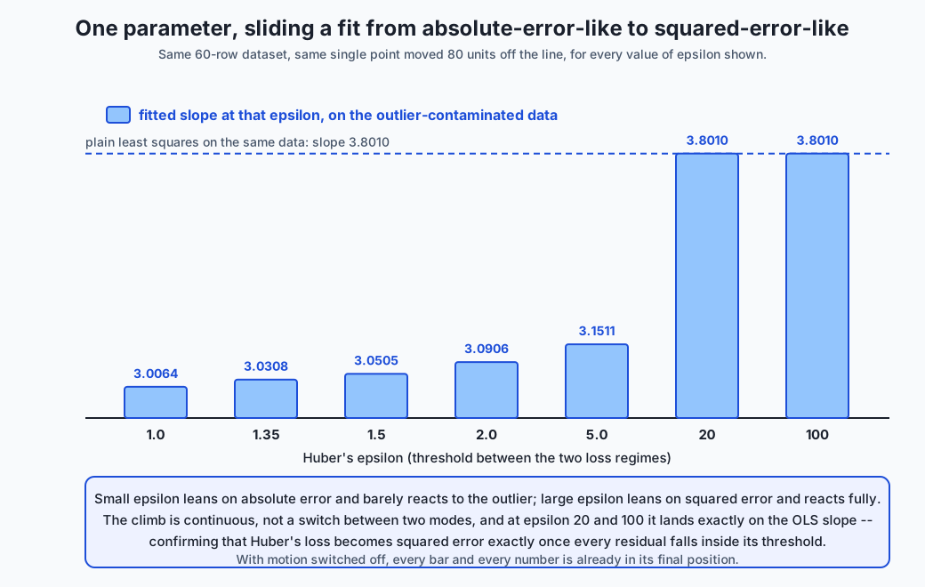
This lesson’s lab moves one point 80 units off a line and then fits
HuberRegressor at seven different values of epsilon on that
contaminated data:
| epsilon | fitted slope |
|---|---|
| 1.0 | 3.0064 |
| 1.35 (scikit-learn’s default) | 3.0308 |
| 1.5 | 3.0505 |
| 2.0 | 3.0906 |
| 5.0 | 3.1511 |
| 20.0 | 3.8010 |
| 100.0 | 3.8010 |
The slope climbs smoothly and monotonically as epsilon grows, and at epsilon 20 and epsilon 100 it lands exactly on 3.8010 — the plain ordinary-least-squares slope on the identical contaminated data. That is not approximate agreement; it is exact, to four decimal places, because once epsilon is large enough that every residual in the dataset falls inside the threshold, Huber’s loss becomes squared error in every single term, with nothing left over from the absolute-error half. Small epsilon leans almost entirely on the outlier-resistant half of the blend; large epsilon collapses back to plain least squares. One parameter, one continuous dial.
The Gauss-Markov theorem, stated precisely
Gauss-Markov is one of the most frequently misquoted results in applied statistics, almost always by dropping one of its qualifying words. Stated in full: under a specific set of assumptions about the errors — linearity of the relationship, unbiasedness of the errors, constant error variance, and no correlation between errors — ordinary least squares is the best linear unbiased estimator.
Every one of those four words is load-bearing. “Best” here means lowest variance, not lowest bias and not lowest error by every conceivable measure. “Linear” restricts the comparison to estimators that are themselves linear combinations of the observed target values — it says nothing about how OLS compares to a nonlinear estimator. “Unbiased” restricts the comparison further, to estimators that are correct on average — it says nothing about how OLS compares to an estimator that deliberately trades a little bias for a lot less variance, which is precisely what ridge regression does on Day 151. And the entire claim is conditional on those four assumptions about the errors holding in the first place.
That conditionality is not a footnote — it is the whole practical
content of the theorem, and it is directly measurable. This lesson’s lab
fits both LinearRegression and HuberRegressor 500 times each on
independently generated data with a known true slope of 3.0, once with
Gaussian errors and once with heavy-tailed errors (a Student’s t
distribution with 3 degrees of freedom, scaled to a similar central
spread):
| errors | OLS mean | OLS spread (sd) | Huber mean | Huber spread (sd) | tighter estimator |
|---|---|---|---|---|---|
| Gaussian | 2.998 | 0.0560 | 2.9977 | 0.0588 | OLS (ratio 0.9524) |
| heavy-tailed | 2.9967 | 0.0589 | 2.9984 | 0.0422 | Huber (ratio 1.3957) |
Both estimators stay within 0.01 of the true value of 3.0 in both settings — neither is biased, in either regime, and that is worth noticing before anything else. What changes is the spread: under Gaussian errors, OLS’s standard deviation across the 500 fits is smaller than Huber’s, exactly as Gauss-Markov promises. Under heavy-tailed errors, the ranking flips — Huber becomes the tighter, more precise estimator, because Gauss-Markov’s assumptions about the errors no longer hold, and its guarantee simply does not apply once they break. The theorem was never wrong; the measurement is showing you the edge of where it applies, not a contradiction of it.
An everyday analogy
Picture a small delivery company trying to answer one question: what is our typical delivery time, and how should one wildly late delivery count toward that number?
Ninety-nine deliveries arrive close to on time, clustered tightly around thirty minutes. The hundredth gets stuck behind an accident and takes four hours. Report the mean of all hundred and that one delivery drags the “typical” time up substantially — the mean has no way to discount a single extreme value; it treats every minute of lateness as equally informative, whether it comes from ordinary traffic or a genuine accident, and a number that large contributes disproportionately just by existing. Report the median instead and the four-hour outlier contributes exactly one vote, identical in weight to a delivery that was one minute late — the median only cares that the outlier is on the late side, never by how much.
Squared-error regression is the mean’s cousin: it inherits exactly the same sensitivity, for exactly the same reason — squaring the accident’s enormous residual turns it into an enormous term in the total, and the fitting procedure will contort the rest of its predictions to shrink that one term. Absolute-error regression is the median’s cousin, for the matching reason: no squaring, no escalation, one bad delivery counts once. And Huber regression is the dispatcher who says, sensibly, “if you’re a few minutes off, I’ll track that precisely — every minute matters for planning. If you’re four hours off, something unusual happened, and I’m not going to let that one event dominate my sense of what a normal day looks like.” That dispatcher’s judgment call — where does “a few minutes” end and “something unusual” begin — is exactly Huber’s epsilon, and this lesson’s sweep of it, from a slope of 3.0064 at epsilon 1.0 up to the exact OLS value of 3.8010 at epsilon 20, is the dispatcher gradually loosening that threshold until every delivery, including the four-hour one, gets treated as perfectly ordinary.
Examples in practice
The five-number grid search
Five values — 2.0, 3.0, 5.0, 7.0, 100.0 — and two questions: which
single number minimises the total squared error against them, and which
minimises the total absolute error. A brute-force numerical search over
a fine grid of candidates, checked against no formula at all, lands at
23.39975 for the first (the true mean is 23.4000) and 5.00005 for the
second (the true median is 5.0000). The single value of 100.0 pulls the
mean to nearly five times the median’s value, purely because it is being
squared into the total.
The loss landscape, swept and measured
Take a real sixty-row dataset and sweep a candidate slope from 2.0 to 4.0, holding the intercept fixed, totalling both losses at each candidate. Both landscapes are minimised at the identical slope of 3.0 on this dataset — the two losses agree completely on the easy case, with no outlier present. What differs is the shape: squared error’s second differences have a standard deviation of exactly 0.000000 (a parabola); absolute error’s have a standard deviation of 1.9366 (kinked). That is the direct, numerical version of “smooth versus piecewise-linear” — not an analogy, a measurement.
The normal equations, solved by hand
On a 300-row dataset, solving (X^T X) beta = X^T y directly with
numpy.linalg.solve gives an intercept of 4.966335126423676 and a
slope of 2.977853013652841. Fitting LinearRegression on the identical
data gives 4.966335126423733 and 2.977853013652829. The two disagree in
the thirteenth decimal place — pure floating-point rounding, not a real
difference — because they are two different arithmetic routes to the
same exact mathematical answer.
The centrepiece: one outlier, three fits
Sixty rows, an ordinary line, and then one point moved 80 units off it:
| estimator | loss it minimises | slope before | slope after | movement |
|---|---|---|---|---|
LinearRegression | squared error | 3.0465 | 3.8010 | +0.7545 |
HuberRegressor | Huber (blended) | 2.9870 | 3.0308 | +0.0437 |
QuantileRegressor(0.5) | absolute error | 2.9961 | 3.0064 | +0.0104 |
The same single corrupted row, the same sixty data points otherwise, and three genuinely different reactions — a seventeen-fold difference between OLS and Huber, and a seventy-two-fold difference between OLS and the median fit. This is not three algorithms disagreeing about how to compute the same answer; it is three different definitions of “the best answer,” disagreeing about what the answer even is.
Implications: security, privacy, performance, scalability, and cost
Security. A pipeline fit with plain squared error on data an attacker can partially influence — a user-submitted rating, a crowd-sourced price feed, a review score — inherits an unbounded sensitivity to any one adversarial value. This lesson’s measured 0.7545 movement from a single corrupted row is a direct illustration: an attacker does not need to control much of your data to move your model substantially, only one value, and squared error hands that one value maximal leverage. Huber and quantile losses put an explicit, tunable ceiling on how much any single point can buy, which is worth treating as a security property, not merely a statistical nicety, whenever a pipeline ingests data it does not fully control.
Privacy. A squared-error fit’s heavy reliance on its most extreme points means those points can disproportionately influence the fitted line — which, in a setting where a model’s parameters or predictions are exposed, can leak more about an unusual individual data point than about the population as a whole. A model that reacts moderately to any single row, as Huber and quantile fits do here, leaks correspondingly less about that row specifically. This is a secondary consideration for the outlier-sensitivity property measured throughout this lesson, not this lesson’s primary subject, but it is worth flagging as one place these two topics touch.
Performance and scalability. The normal equations are a single
linear-algebra solve — fast, exact, and well-understood at scale via
standard numerical libraries, though the direct (X^T X) inversion used
here becomes numerically less stable as the number of predictor columns
grows, which Day 150’s multiple-predictor setting will address more
carefully. Huber and quantile regression, by contrast, both require
iterative solvers — HuberRegressor’s reweighted approach and
QuantileRegressor’s linear program — meaning more compute per fit and,
for very large datasets, meaningfully slower training. Choosing a robust
loss is not free; it is a real computational trade against outlier
protection, and the trade gets more expensive as the dataset grows.
Cost. On the datasets in this lesson’s lab — tens to hundreds of rows — the difference between a closed-form solve and an iterative robust fit is a matter of milliseconds, immaterial to any real budget. At production scale, with millions of rows and features fit repeatedly during hyperparameter search, an iterative robust loss can meaningfully add to compute cost, and that cost should be weighed against how much outlier protection the data actually needs — not assumed to be free, and not assumed to be prohibitive without checking.
Alternatives: free, open source, and commercial
scikit-learn (LinearRegression, HuberRegressor,
QuantileRegressor) — free and open source under the BSD 3-clause
licence, and the tool used throughout this lesson’s lab. LinearRegression
is the right default when you have checked for outliers and found none
of concern, or when speed matters and the closed form’s exactness is
worth more than robustness. HuberRegressor is the right choice when
you expect occasional bad rows but still want most of squared error’s
statistical efficiency on the well-behaved majority; its one knob,
epsilon, is the threshold swept in this lesson’s animated diagram.
QuantileRegressor(quantile=0.5) is the right choice when you want the
strongest available protection against extreme values and can accept the
computational cost of an iterative linear-program solve; it also
generalises past the median, to any quantile, which Day 152’s cousin
concepts around prediction intervals will touch on. All three were used
directly in this lesson, and their behaviour is measured, not asserted.
statsmodels — also free and open source, and worth knowing about
because it offers sm.OLS alongside sm.RLM (robust linear models,
including a Huber-style M-estimator) with a heavier emphasis on
statistical inference — standard errors, confidence intervals and
hypothesis tests reported by default, in a style closer to traditional
econometrics than scikit-learn’s prediction-first API. Described here
from its documentation; no output from statsmodels is reproduced
anywhere in this lesson or its lab.
R’s built-in lm() and the MASS package’s rlm() — free, open
source under GPL, and the long-standing default toolkit in academic
statistics. lm() fits ordinary least squares via the normal equations,
identically in spirit to this lesson’s own hand-solved version; rlm()
fits Huber-style robust regression. Described here from documentation
only; this course’s labs are Python-based and no R output is reproduced.
SAS’s PROC ROBUSTREG — a commercial, paid product, part of SAS’s
enterprise analytics suite, offering several robust-regression methods
including M-estimation (the Huber family) and least-trimmed-squares.
Licensing is typically per-seat or per-server and priced through direct
SAS sales rather than published list pricing, so no specific figure is
quoted here; scikit-learn’s HuberRegressor and QuantileRegressor,
both used directly in this lesson, are free, well-documented equivalents
for the core ideas this lesson covers.
Comparison with related concepts
Loss versus penalty. A loss scores how well a candidate fits the data; a penalty, added on top of a loss, additionally discourages large coefficients regardless of fit. Ridge and lasso (Day 151) are squared error plus a penalty — the loss underneath is unchanged, and everything this lesson measured about squared error’s outlier sensitivity still applies to a ridge or lasso fit unless a robust loss is substituted in as well. The two ideas are independent design axes, not alternatives to each other.
Loss versus metric, restated once more because it is easy to blur:
optimised during fitting versus reported afterward, and not required to
be the same function. This lesson’s HuberRegressor fits by minimising
Huber loss and could equally be reported using mean absolute error,
root mean squared error, or R-squared — Day 152’s subject, deliberately
left untouched here beyond this one clarifying sentence.
Squared and absolute error versus classification losses. Fitting a line and fitting a classifier both work by minimising a loss, but the losses look different because the targets do: log loss and hinge loss, which a future course day covers, score a probability or a margin rather than a numeric residual. The underlying principle — a loss is a choice, and the choice has consequences — carries over identically; the specific formulas do not.
Robust regression versus outlier removal. A tempting alternative to any of this lesson’s losses is simply deleting rows that look extreme before fitting anything. That approach requires deciding, by some other rule, what counts as “extreme” — a judgment call made once, by hand, before seeing how it affects the fit. Huber and quantile regression make that judgment continuous and principled instead: every row stays in the data, and the loss itself determines how much influence it gets, rather than a binary keep-or-discard decision made in advance.
When to use it — and when not to
Use plain squared error (LinearRegression) when you have genuinely
checked for outliers and found the data reasonably well-behaved, and
when the extra statistical efficiency it offers under those conditions —
measured directly in this lesson as a smaller standard deviation across
repeated fits — is worth having. It is also the right choice whenever
speed and exactness matter more than robustness: the normal equations
give you a single, exact, and fast answer with no iteration.
Use Huber loss when you expect occasional bad rows but do not want to throw away statistical efficiency on the well-behaved majority. Its one tunable knob lets you decide, explicitly, how large a residual has to get before it stops being treated as “ordinary” — this lesson’s sweep, from 3.0064 at epsilon 1.0 to the exact OLS answer of 3.8010 at epsilon 20, is a direct picture of that knob’s whole range.
Use quantile regression at the median when you want the strongest practical protection against extreme values, or when you specifically want to estimate a conditional median rather than a conditional mean — a genuinely different quantity whenever the target’s distribution is skewed. Accept, in exchange, a slower iterative fit and somewhat less statistical efficiency on well-behaved data.
Do not reach for a robust loss reflexively, on every dataset, regardless of what the data looks like. This lesson’s own measurement shows OLS winning the precision contest under Gaussian errors — Huber was, on that specific comparison, the worse choice. Robustness is a real trade, not a strict upgrade: it buys protection against extreme values at a real cost in statistical efficiency when those extreme values never actually show up. Look at the data — or, better, measure both losses on it, the way this lesson’s lab does — before deciding which loss to minimise.
The AI thread
The mechanism this lesson measured — squaring gives one extreme value disproportionate leverage — is not confined to fitting a straight line to sixty rows. It is present, in some form, in essentially every model trained by minimising an average loss over a dataset, and AI practice runs into it in at least three recognisable places.
Reward models and preference data. A reward model in reinforcement learning from human feedback is fit, in large part, by minimising some loss over human-provided scores or comparisons. A rater who is inconsistent, adversarial, or simply has an unusual day contributes a residual just like this lesson’s single corrupted delivery, and a squared-error-style objective will let that one rater’s disagreement pull the reward model’s behaviour further than a robust objective would. Practitioners who down-weight or clip extreme disagreements between raters are, whether or not they use that language, making exactly the choice this lesson names explicitly.
Data poisoning. A model whose training loss reacts strongly to a single extreme example is more exploitable by an adversary who can inject even one bad example into a training or fine-tuning set — this lesson’s 0.7545-versus-0.0104 comparison is a direct, if simplified, illustration of how much leverage that one example can be handed, purely as a consequence of which loss the pipeline minimises. This is not a theoretical concern confined to linear regression; the same squaring mechanism is present, with the same qualitative effect, in the loss functions behind much larger models.
Evaluation and benchmark aggregation. When a benchmark score is computed as a mean across many examples, one anomalous example — a malformed prompt, a scoring bug on a single item — can shift the reported number disproportionately, exactly as this lesson’s 100.0 shifted the mean of five numbers to nearly five times the median. Median or trimmed-mean aggregation, borrowed directly from this lesson’s robust-loss intuition, is a standard and underused defence.
None of this requires a different mental model from the one this lesson built with sixty rows and a straight line. The scale changes; the mechanism — squaring rewards large deviations disproportionately, and that reward can be exploited or simply triggered by accident — does not.
Knowledge check
- Explain, in your own words and without looking anything up, why the
mean minimises squared error and the median minimises absolute error.
Use the values
2.0, 3.0, 5.0, 7.0, 100.0in your explanation. - Sweeping a candidate slope produces a squared-error curve with constant second differences and an absolute-error curve with varying second differences. Connect that fact directly to why one loss has a closed-form solution (the normal equations) and the other does not.
- A single point is moved 80 units off a fitted line. State, in one sentence, the arithmetic reason ordinary least squares reacts far more than a Huber fit does.
- Huber’s epsilon parameter is swept and the fitted slope converges exactly to the OLS answer at large epsilon. Explain why “exactly” rather than merely “approximately.”
- State the Gauss-Markov theorem with all four of its qualifying words present, and explain what each word rules out.
- Under Gaussian errors, OLS’s standard deviation across 500 fits is smaller than Huber’s. Under heavy-tailed errors, the ranking flips. Explain why this is not a contradiction.
- A model is fit by minimising squared error and reported using mean absolute error. Is this a mistake? Justify your answer using the distinction between a loss and a metric.
- Name one setting in AI practice, other than the ones this lesson named, where a squared-error-style loss could give an outlier or an adversarial example disproportionate influence.
Hands-on exercise
Today’s lab, Loss Functions and Least Squares, measures every claim in
this lesson directly, on real (synthetic, seeded) data: the mean and
median as minimisers, the smooth-versus-kinked landscape shapes, the
normal equations matching LinearRegression, the outlier-shift table,
the Huber epsilon sweep, and the Gauss-Markov efficiency comparison
under both Gaussian and heavy-tailed errors.
Ten exercises. The first four rebuild the calculus (what each loss minimises, and why one has a closed form). The next three measure outlier sensitivity directly, including the epsilon sweep. The last two measure Gauss-Markov’s conditional promise under two different error distributions.
Build the environment, then work through starter/test_loss_claims.py,
replacing one pytest.skip at a time.
Expected output
The harness ends with:
---------------------------------------------------------------
14 checks, 0 failure(s)
and exits 0. pytest examples -q reports 14 passed, and
pytest starter -q reports 4 passed, 10 skipped until you begin.
The measured table includes:
  estimator    before     after    movement
  ols        3.0465    3.8010    +0.7545
  huber      2.9870    3.0308    +0.0437
  quantile   2.9961    3.0064    +0.0104
  Gaussian errors     : OLS mean=2.9980 sd=0.0560   Huber mean=2.9977 sd=0.0588
  heavy-tailed errors : OLS mean=2.9967 sd=0.0589   Huber mean=2.9984 sd=0.0422
Validate your work
bash tests/run_tests.sh; echo "exit=$?"reports14 checks, 0 failure(s)andexit=0. Capture the harness’s own exit status..venv/bin/pytest examples -qreports14 passed..venv/bin/python3 examples/report_measurements.py | diff - expected-output/measured-values.txtproduces no output.- When you have finished every exercise,
pytest starter -qreports14 passed. - Break one assertion on purpose, confirm the harness fails, restore it.
Troubleshooting
import file mismatch. You ran pytest examples starter together.
Run them separately, always — both directories define modules with the
same names.
Your numbers in the later exercises differ slightly. Read
expected-output/FIELDS.md first. Everything past the normal-equations
exercise is sampled, from numpy.random.default_rng or from an
iterative scikit-learn solver, and neither carries a cross-version
guarantee. What must hold on any version: OLS moves furthest of the
three estimators under an outlier, the epsilon sweep is non-decreasing,
and Gaussian errors favour OLS while heavy-tailed errors favour Huber.
QuantileRegressor raised a solver error. This lab passes
solver="highs" explicitly; if you build your own without naming a
solver, check which one your scikit-learn version defaults to.
The efficiency comparison takes a noticeable moment. It fits 2,000 models in total. No timing is asserted anywhere, so a slow machine changes nothing about whether the checks pass.
Common mistakes
Treating “the mean” as a natural default rather than squared error’s minimiser. The grid search in exercise 1 finds the mean without ever computing an average — it discovers it from the loss’s own definition, which is the point.
Describing Huber as “the robust one” without naming its epsilon parameter. It is a one-parameter family with OLS-like behaviour at one end and MAE-like behaviour at the other, not a fixed alternative to either.
Concluding from the heavy-tailed result alone that Huber is simply better. Exercise 6 measured OLS winning under Gaussian errors. Run both before drawing a conclusion.
Reciting Gauss-Markov without its qualifying words. “Best” (lowest variance), “linear,” “unbiased,” and conditional on its assumptions are all load-bearing; dropping any of them changes what is being claimed.
Practice assignment
Take a regression you have already fit, or one you can fit quickly on data you have on hand.
- Fit it with both a squared-error loss and a robust loss — OLS and
HuberRegressor, at minimum. Do not decide in advance which is “right”; measure both. - Deliberately corrupt one row by a large, obvious amount — the way this lesson moved one point 80 units off its line — and refit both models. Report how far each coefficient moved, and the ratio between the two movements.
- Sweep Huber’s epsilon on your corrupted data across at least five values, and report whether the sweep is monotonic and where it converges.
- Check whether your data looks more Gaussian or more heavy-tailed by plotting a histogram of your model’s residuals (fit without the deliberate corruption). State, based on that shape alone, which loss you would predict wins the precision contest, then check your prediction against the corrupted-vs-uncorrupted comparison you just ran.
- Write one paragraph stating which loss you would ship for this specific dataset, and why — citing the numbers from steps 1 through 4, not a general preference.
The deliverable is the comparison, not a single “correct” model.
Extension challenge
Pick one and measure it.
- Ridge, ahead of schedule. Fit
Ridge(alpha=1.0)on this lesson’s outlier-contaminated dataset and compare its coefficient movement to plainLinearRegression’s. Day 151 owns penalties properly; this is a preview of how a penalty interacts with an unchanged loss. - A second heavy tail. Repeat the Gauss-Markov comparison with a Laplace-distributed error instead of Student’s t, and report whether the efficiency ranking still flips in Huber’s favour.
- Find the crossover. Sweep the degrees of freedom of the Student’s t error from 30 down to 1 and estimate, approximately, the point at which OLS and Huber’s standard deviations cross. Report what that implies about how heavy the tails need to be before Huber earns its keep.
- Two outliers. Add a second point 80 units off the line at a different predictor value, and re-measure the outlier-shift table. Does OLS’s movement roughly double, or is the effect worse than linear?
- Beyond the median. Fit
QuantileRegressoratquantile=0.1andquantile=0.9on the outlier-contaminated data, and describe, in one paragraph, what the gap between those two fitted lines tells you that a single squared-error fit cannot.
Quiz
Q1. A grid search over sum((v - c)^2) for the values [2.0, 3.0, 5.0, 7.0, 100.0] lands at 23.39975. The true mean is 23.4. What does this experiment actually demonstrate?
- That the mean IS the minimiser of squared error -- not chosen for it by convention, but the number that falls out of the calculus
- That the grid search has a bug, since the mean should not depend on a single value like 100.0
- That squared error is the wrong loss to use whenever an outlier is present
- That the grid needed to be finer to find the exact minimiser
Show answer
Answer: A. That the mean IS the minimiser of squared error -- not chosen for it by convention, but the number that falls out of the calculus
The mean is not a natural summary that squared error happens to agree with -- it is the exact quantity you get by setting the derivative of sum-of-squares to zero and solving. The grid search finds this without ever computing an average, which is the point: it is discovering the mean, not confirming a formula. The mean genuinely IS pulled toward 100.0 (that is squared error's known property, not a bug), and while a finer grid gets closer to 23.4 exactly, the 0.00025 gap here is expected grid resolution, not evidence of anything broken.
Q2. Sweeping a candidate slope produces a squared-error curve whose second differences have standard deviation 0.000000, and an absolute-error curve whose second differences have standard deviation 1.9366. What does that contrast explain?
- That squared error is more accurate than absolute error at finding the true slope
- That squared error's landscape is a smooth parabola (constant curvature) while absolute error's is piecewise-linear with kinks -- which is exactly why one has a closed-form solution and the other does not
- That absolute error is a buggier implementation than squared error in this library
- Nothing about the fitting itself -- second differences are only a numerical curiosity
Show answer
Answer: B. That squared error's landscape is a smooth parabola (constant curvature) while absolute error's is piecewise-linear with kinks -- which is exactly why one has a closed-form solution and the other does not
A constant second difference is the numerical signature of a parabola -- one smooth minimum, differentiable everywhere. A varying second difference means the curve is a sequence of straight segments meeting at kinks, which is what absolute error's landscape actually looks like. This directly explains the normal equations: they exist because squared error's derivative is defined everywhere and can be set to zero and solved, which is not available for a function with a corner. Neither curve says anything about which loss finds a more "accurate" slope on this particular dataset -- both landscapes were minimised at the identical slope here.
Q3. Moving one point 80 units off a fitted line moves an ordinary-least-squares slope by 0.7545, a Huber fit's slope by 0.0437, and a median-regression fit's slope by 0.0104. What is the mechanism behind that seventeen-to-seventy-two-times difference?
- HuberRegressor and QuantileRegressor use a different, more accurate optimizer than LinearRegression
- The three estimators were fit on different subsets of the same data
- Squaring the 80-unit residual makes it contribute 6,400 to the total loss, so the optimizer distorts the rest of the fit substantially to shrink that one term; absolute error only contributes 80, and Huber caps the contribution beyond its threshold
- LinearRegression has a bug that the other two estimators do not share
Show answer
Answer: C. Squaring the 80-unit residual makes it contribute 6,400 to the total loss, so the optimizer distorts the rest of the fit substantially to shrink that one term; absolute error only contributes 80, and Huber caps the contribution beyond its threshold
All three estimators are fit on the identical sixty rows, including the identical moved point, so neither differing data nor differing optimizer quality is the explanation. The mechanism is arithmetic: squaring turns a residual of 80 into a term of 6,400 in the total loss, so minimising that total means trading away a great deal of fit elsewhere to shrink the one huge squared term. Absolute error keeps that same residual's contribution at 80 -- proportional, not squared -- and Huber caps a large residual's contribution once it passes its threshold, whichever regime it uses.
Q4. Huber's epsilon parameter is swept from 1.0 to 100.0 on outlier-contaminated data and the fitted slope climbs smoothly from 3.0064 to 3.8010, landing exactly on the plain-least-squares answer at the high end. What does that describe?
- A bug: HuberRegressor should never reproduce LinearRegression exactly
- Epsilon controls how many iterations the solver runs, which happens to correlate with the slope
- The outlier stopped affecting the fit once epsilon passed a certain value
- Huber's loss is squared error inside the threshold and scaled absolute error outside it, so raising the threshold hands progressively more of the loss to the squared-error half -- a continuous interpolation, not a switch between two fixed modes
Show answer
Answer: D. Huber's loss is squared error inside the threshold and scaled absolute error outside it, so raising the threshold hands progressively more of the loss to the squared-error half -- a continuous interpolation, not a switch between two fixed modes
As epsilon grows, fewer and fewer residuals exceed the threshold, so more and more of the loss behaves like squared error -- and in the limit, every residual falls inside the threshold and Huber's loss becomes squared error exactly, which is why the sweep converges precisely to the OLS slope rather than merely approaching it. This is a genuine one-parameter family, not two discrete behaviours with a cutover, and the outlier is never excluded -- it is just weighted less severely as epsilon shrinks.
Q5. The Gauss-Markov theorem says ordinary least squares is the "best linear unbiased estimator." Which reading of that phrase is correct?
- Among estimators that are LINEAR in the observed y values and UNBIASED, OLS has the lowest variance -- a claim conditional on its assumptions, saying nothing about nonlinear or biased alternatives, or about what happens if the assumptions do not hold
- 'Best' means OLS achieves zero variance under its assumptions
- OLS has the lowest possible error of any estimator, linear or not, under any error distribution
- OLS is unbiased, and separately, it happens to also be the fastest algorithm to compute
Show answer
Answer: A. Among estimators that are LINEAR in the observed y values and UNBIASED, OLS has the lowest variance -- a claim conditional on its assumptions, saying nothing about nonlinear or biased alternatives, or about what happens if the assumptions do not hold
Every qualifying word restricts the claim: LINEAR excludes anything like Huber that is not a simple linear combination of y; UNBIASED excludes estimators that trade some bias for lower variance; and the whole statement is conditional on Gauss-Markov's assumptions about the errors. It is not a claim that OLS beats every possible estimator, and it says nothing about what happens once those assumptions are violated -- which is exactly what the heavy-tailed experiment in this lesson tests.
Q6. Over 500 replications with a true slope of 3.0, Gaussian errors give OLS a standard deviation of 0.0560 against Huber's 0.0588, while heavy-tailed errors give OLS 0.0589 against Huber's 0.0422. Both estimators' means stay within 0.01 of 3.0 in both settings. What is the correct conclusion?
- Huber is unbiased and OLS is biased under heavy-tailed errors
- OLS is more precise under Gaussian errors and Huber is more precise under heavy-tailed errors; both remain roughly unbiased throughout -- the ranking that changes is PRECISION, not correctness on average
- The results are contradictory and one of the two experiments must contain an error
- Huber should always be preferred, since it is closer to OLS under Gaussian errors and better under heavy-tailed errors
Show answer
Answer: B. OLS is more precise under Gaussian errors and Huber is more precise under heavy-tailed errors; both remain roughly unbiased throughout -- the ranking that changes is PRECISION, not correctness on average
Both means staying within 0.01 of 3.0 in both settings is the evidence that bias is not what changed -- both estimators track the truth on average, in both error regimes. What changed is the spread: OLS's standard deviation is smaller under Gaussian errors (Gauss-Markov's promise holding), and Huber's is smaller under heavy-tailed errors (Gauss-Markov's promise no longer applying, since its assumptions were violated). The two results are not contradictory; they are the same experiment measuring the same conditional claim under two different conditions. And "always prefer Huber" ignores that it lost the Gaussian comparison.
Q7. This lesson repeatedly measures a "loss," while a later day covers "metrics." What is the distinction, stated precisely?
- A loss applies only to regression, and a metric applies only to classification
- A metric is always a rescaled version of the loss the model was fit with
- A loss is what an algorithm optimises during fitting; a metric is what you report to judge the result -- and they need not be the same function, so a model can be FIT with one and REPORTED with another
- A loss and a metric are two names for the same idea, used interchangeably by convention
Show answer
Answer: C. A loss is what an algorithm optimises during fitting; a metric is what you report to judge the result -- and they need not be the same function, so a model can be FIT with one and REPORTED with another
They serve different jobs and can diverge freely: a model fit by minimising squared error is routinely reported using mean absolute error or R squared, and a model fit with Huber loss can be reported with root mean squared error. Neither is restricted to one task type -- absolute and squared losses both apply to regression here, and classification has its own losses and metrics that follow the identical split. Treating them as interchangeable, or assuming the report is always a rescaling of the objective, misses why the two exist as separate concepts.
Q8. Before building any exercise on HuberRegressor and QuantileRegressor, this lab's author checked that both estimators exist and converge without warning in the pinned scikit-learn release. Why does that check matter, as a matter of intellectual honesty rather than mere caution?
- It matters only for performance reasons, not correctness
- It doesn't matter much -- any reasonably recent scikit-learn version supports every estimator ever documented
- It was unnecessary, since QuantileRegressor has been part of scikit-learn since its very first release
- Because assuming a tool's behavior from memory or from another version's documentation, rather than verifying it against the actual pinned version, is exactly the kind of unearned claim this course's measured-not-asserted standard exists to prevent
Show answer
Answer: D. Because assuming a tool's behavior from memory or from another version's documentation, rather than verifying it against the actual pinned version, is exactly the kind of unearned claim this course's measured-not-asserted standard exists to prevent
Estimator APIs, defaults and even availability change between scikit-learn releases -- QuantileRegressor is a comparatively recent addition, and solver defaults have changed across versions. Writing an exercise around behavior that was never actually run against the pinned version would be exactly the fabricated-output problem this course is built against, just relocated from a data claim to a tool claim. The fix is the same either way: run it, watch it converge, and only then build on it.
Glossary
- Loss function
- A rule that turns one candidate line's residuals into a single number to minimise. Not a fixed property of "doing regression" -- a choice, made explicitly here between squared error, absolute error and a blend of the two.
- Squared error
- The loss `sum((y - prediction)^2)`. Minimised by the mean; smooth everywhere, with one minimum; squares every residual, so an 80-unit error contributes 6,400 to the total, seventeen to seventy-two times more than the loss below moves for the same outlier.
- Absolute error
- The loss `sum(|y - prediction|)`. Minimised by the median; piecewise-linear, with a kink at every point where a residual crosses zero; has no closed-form minimiser because its derivative does not exist at a residual of exactly zero.
- Mean squared error
- Squared error divided by the row count. The per-row average of the loss actually minimised; distinct from root mean squared error, which is a metric reported in the target's own units -- Day 152's subject, not this lesson's.
- Normal equations
- The closed-form solution to squared-error linear regression, `(X^T X) beta = X^T y`, obtained by setting the loss's derivative to zero and solving. Measured here to match `LinearRegression` to within 6e-14.
- Huber loss
- A loss that is squared error inside a threshold `epsilon` and (scaled) absolute error outside it. Continuous, not a hard switch: sweeping epsilon from 1.0 to 100.0 moved the fitted slope smoothly from 3.0064 to 3.8010, the exact OLS answer on the same data.
- Quantile regression
- Regression that minimises a loss asymmetric around one target quantile. At quantile 0.5 it minimises absolute error and estimates the conditional median; scikit-learn's `QuantileRegressor(quantile=0.5, alpha=0.0)` is what this lesson used for that case.
- Outlier sensitivity
- How far an estimator's fit moves in response to one extreme point. Measured directly here: moving a single point 80 units off the line moved OLS's slope by 0.7545, Huber's by 0.0437 and the median fit's by 0.0104.
- Robust regression
- Any regression method designed to bound the influence of extreme points, typically by using a loss that grows slower than squared for large residuals. Huber and quantile regression are both robust in this sense; ridge and lasso, covered on Day 151, are not -- they change the penalty, not the loss's shape.
- Gauss-Markov theorem
- Under linearity, unbiasedness of the errors, constant error variance and no correlation between errors, ordinary least squares is the best linear unbiased estimator -- lowest variance among estimators that are linear in y and unbiased. Every qualifying word is load-bearing; the guarantee is conditional on those assumptions, not universal.
- Best linear unbiased estimator (BLUE)
- The specific claim Gauss-Markov makes about OLS: among all estimators that are (a) linear combinations of the observed y values and (b) correct on average, OLS has the smallest variance. It says nothing about estimators that are nonlinear or biased, some of which can do better -- which is exactly what Huber demonstrated under heavy-tailed errors here.
- Statistical efficiency
- How small an unbiased estimator's variance is, relative to alternatives. Measured here as the ratio of two standard deviations across 500 replications: 0.9524 in OLS's favour under Gaussian errors, 1.3957 in Huber's favour under heavy-tailed errors.
- Heavy-tailed distribution
- A distribution whose extreme values occur far more often than a Gaussian's. Constructed here with a Student's t distribution at 3 degrees of freedom, scaled to a similar central spread as the Gaussian comparison, so the two settings differ only in how often big errors occur.
- Unbiasedness
- An estimator's average value, over many independent datasets, equals the true parameter. Confirmed separately from efficiency here: both OLS and Huber stayed within 0.01 of the true slope of 3.0 in both error settings, so bias was never what changed between them.
- Loss versus metric
- A loss is the function an algorithm optimises during fitting; a metric is the function you report to judge the result. They need not be the same function -- a model can be fit with squared error and reported with mean absolute error, or fit with Huber and reported with R squared. Day 152 owns metrics as a subject.
- Convex loss
- A loss whose landscape has no separate local minima to get trapped in -- squared error, absolute error and Huber are all convex in the model's coefficients, which is part of why the normal equations and iterative solvers alike reliably find the global minimum.
- Differentiability
- Whether a function has a well-defined slope at every point. Squared error is differentiable everywhere, which is what makes the normal equations possible; absolute error is not differentiable at a residual of zero, which is why it has no equivalent closed form.
- Second difference
- The discrete analogue of a second derivative: `diff(diff(values))`. Constant across a swept squared-error curve here (standard deviation 0.000000, a parabola); varying across the matching absolute-error curve (standard deviation 1.9366, a kinked, piecewise-linear shape).
Sources and further reading
- Linear Models -- scikit-learn user guide, including ordinary least squares, Huber and quantile regression — scikit-learn developers (accessed 2026-08-27)
- LinearRegression -- scikit-learn API reference — scikit-learn developers (accessed 2026-08-27)
- HuberRegressor -- scikit-learn API reference — scikit-learn developers (accessed 2026-08-27)
- QuantileRegressor -- scikit-learn API reference — scikit-learn developers (accessed 2026-08-27)
- Gauss-Markov theorem — Wikipedia (accessed 2026-08-27)
- Ordinary least squares — Wikipedia (accessed 2026-08-27)
- Huber loss — Wikipedia (accessed 2026-08-27)
- The Elements of Statistical Learning, chapter 3 on linear methods for regression -- free PDF from the authors — Trevor Hastie, Robert Tibshirani and Jerome Friedman, Springer (accessed 2026-08-27)
Kept in this browser, no account needed. Your progress page turns the whole record into one link you can bookmark or open on another device.