Machine Learning › Regression › Day 150
Day 150: Multiple and Polynomial Regression

After this lesson you will know what changes the moment a second predictor joins the first, because you will have measured it on real clinical data. You will append an exact copy of a predictor correlated at 0.8967 with another column already in the model, and watch its coefficient of -1.09 split into two coefficients of -0.545 each -- neither matching the original, their sum matching it to eight decimal places, and every prediction the model makes changing by less than four trillionths. You will break that exact tie with one percent of noise and watch the two coefficients swing across a range wider than twelve units and repeatedly change sign, while their sum barely moves and R-squared holds at 0.5177 to 0.5186 across ten different noise draws. You will compute variance inflation factors directly from their definition on ten real predictors, from 1.22 for age to 59.20 for a serum measurement, and confirm with bootstrap resampling that the high-VIF predictors are the unstable ones. You will watch a predictor's coefficient flip sign between a simple regression and a multiple one -- positive alone, negative once a correlated partner is held constant -- on real data, not a constructed example. You will prove that a polynomial fit is linear in its parameters by solving the identical expanded design matrix two different ways and finding the answers agree to thirteen decimal places. And you will measure two quiet failure modes that later days exist specifically to fix: R-squared climbing from 0.5177 to 0.5325 as ten columns of pure noise are added, and standardising a design matrix moving every coefficient by a factor of thirty or more while changing not one prediction.
Hands-on lab for this lesson
Lab files on GitHub: https://github.com/ai-roadmap-365/ai-roadmap-365.github.io/tree/main/labs/sections/machine-learning/day-150-multiple-and-polynomial-regression
- Get the hands-on files. Clone the labs repository once (you can reuse this clone for every lesson). This works on macOS, Linux, and Windows (PowerShell or WSL):
git clone https://github.com/ai-roadmap-365/ai-roadmap-365.github.io.git cd ai-roadmap-365.github.io - Open this lesson's lab. Move into the directory for this specific day. Every lab lives at the same predictable path — section / subsection / week / day:
cd labs/sections/machine-learning/day-150-multiple-and-polynomial-regression - Read the lab guide. Open `README.md` in that directory. It lists the exact commands, what each does, the expected output, and how to check your work — read it before running anything.
- Run it and check your work. Follow the README's "How to run" section: run the example first to see the finished result, then complete the numbered exercises in `starter/`, then run the tests. The tests pass (exit 0) only when your work is correct.
bash tests/run_tests.sh # or the test command named in the lab README
You can also open the lab as a local page (works offline, shows the file tree and expected output).
Learning objectives
By the end of this lesson you will be able to:
- Explain what a coefficient in a multiple regression means, and why "holding the other predictors constant" is doing enormous work in that definition
- Compute variance inflation factors directly from their definition, and read what they say about ten real clinical predictors
- Demonstrate that duplicating a correlated predictor splits its coefficient arbitrarily while conserving the sum and leaving predictions almost untouched
- Distinguish an exact duplicate, which splits its coefficient in a closed-form way, from a near-duplicate, whose split is unstable and effectively arbitrary
- Connect a predictor's variance inflation factor to how much its coefficient wobbles under bootstrap resampling
- Identify a sign flip between a predictor's simple and multiple regression coefficients, and explain the conditioning that caused it
- Build a polynomial design matrix with PolynomialFeatures and explain why the resulting model is still linear in its parameters
- Interpret an interaction term as a claim that one predictor's effect depends on the level of another, distinct from either predictor curving on its own
- Measure that R-squared cannot decrease when a predictor is added, even a column of pure noise, and explain the mechanism
- Measure that standardising a design matrix changes every coefficient's magnitude while leaving every prediction and R-squared unchanged
- State when feature scaling matters for a model and when it does not, for ordinary least squares specifically
- Recognise multicollinearity as a coefficient-interpretation problem, not a prediction-quality problem, and name ridge regression as the standard remedy
Prerequisites
- Day 148 -- the geometry of a line through one predictor, and how to read a single coefficient
- Day 149 -- why squared error is the loss being minimised, and the normal equations that solve for it
- Day 145 -- the capacity-versus-error trade-off measured with polynomial degree; today is about the mechanics of the fit, not that trade-off again
- Day 119 -- Simpson's paradox, which returns here as a coefficient sign flip on real data
- Comfort with NumPy arrays and reading a pytest failure, and a working python3 3.11 or newer on your PATH; the lab builds its own virtual environment and needs no GPU
Why this matters
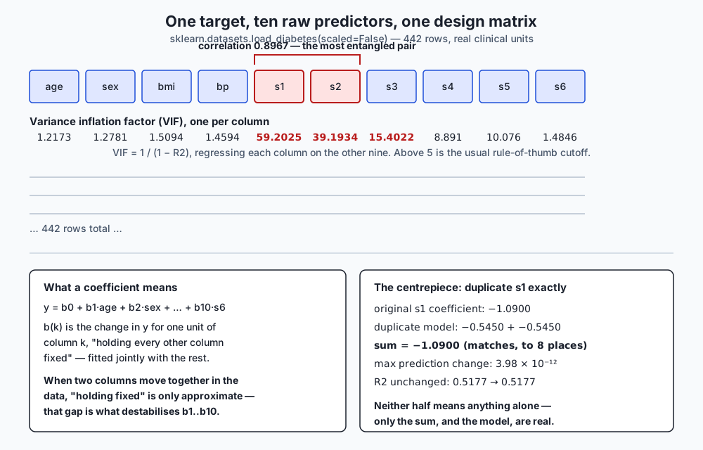
Take one column of real patient data — a serum measurement, s1 — and copy it. Not transform it, not engineer a new feature from it: copy it, byte for byte, and hand the model two columns that say the exact same thing. Refit.
  original s1 coefficient        : -1.0900
  duplicate model, coefficient a : -0.5450
  duplicate model, coefficient b : -0.5450
  sum of the two                 : -1.0900
  max abs prediction difference  : 3.98e-12
  R2 original / duplicate        : 0.5177 / 0.5177
Nothing about the model’s accuracy changed. The predictions moved by four trillionths — noise smaller than a rounding error. R-squared held at 0.5177 to four decimal places on both sides. Whatever this model is worth as a predictor, duplicating a column changed none of it.
But look at the coefficients. -1.09 became two numbers, -0.545 and -0.545, and neither one is the original. Split the effect down the middle and call it a day — reasonable enough, until you notice why it split evenly: the two columns are identical, so nothing distinguishes them, and the normal equations simply picked the tidiest of infinitely many valid splits.
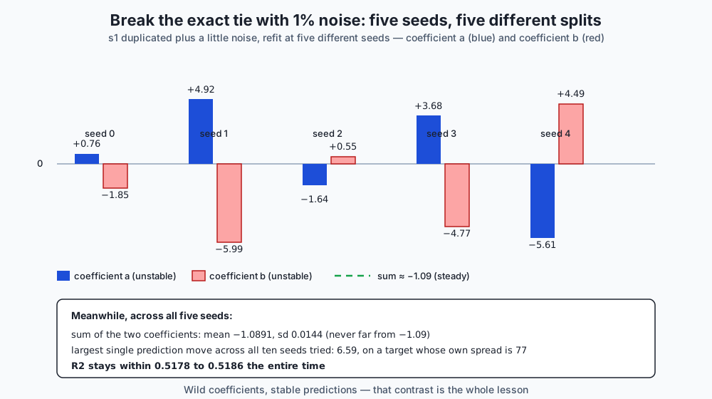
Now break that tie. Add one percent of random noise to the copy — an amount too small to see in a scatter plot — and refit at a few different noise draws:
  seed 0: coefficient a = +0.7592   coefficient b = -1.8451   sum = -1.0859
  seed 1: coefficient a = +4.9238   coefficient b = -5.9881   sum = -1.0643
  seed 2: coefficient a = -1.6402   coefficient b = +0.5508   sum = -1.0893
  seed 3: coefficient a = +3.6831   coefficient b = -4.7727   sum = -1.0896
  seed 4: coefficient a = -5.6134   coefficient b = +4.4931   sum = -1.1203
Read that again. The original coefficient, before any duplication, was -1.09 — negative. At seed 0, one of its two halves is +0.76 — positive, and larger in magnitude than the coefficient it split from. At seed 1, the two halves are +4.92 and -5.99: values five times the size of anything in the honest model, of opposite sign, describing what is essentially the same nine-tenths-correlated pair of columns. Across just five noise draws, one coefficient ranges from -5.61 to +4.92 — an eleven-unit swing on a value that started at -1.09.
And the sum, every single time, sits within 0.03 of -1.09. The predictions barely move at all — across ten noise seeds, the single largest prediction change anywhere in the dataset is 6.59, on a target whose own values span from 25 to 346 with a standard deviation of 77. R-squared holds between 0.5178 and 0.5186 throughout.
Wild coefficients, stable predictions. That is the whole subject of this lesson in one sentence. A model with more than one predictor can be excellent at what it predicts and worthless — actively misleading — as a description of what any individual coefficient means, and nothing about its accuracy, its R-squared, or its predictions will ever tell you so. You have to check the coefficients themselves, and this lesson shows you how.
This matters for AI work specifically because “explainable” model output almost always means “the coefficients, or something coefficient-shaped.” A feature-importance chart, a SHAP value, a linear probe on an embedding, an ablation study reporting “removing this input cost 2 points of accuracy” — every one of these is vulnerable to the exact failure measured above the moment two inputs carry overlapping information, which in any real feature set is most of the time. Understanding multiple regression’s mechanics is the prerequisite for knowing when to trust an explanation and when you are reading noise dressed up as insight.
The idea in plain language
Day 148 gave you a line through one predictor: one input, one coefficient, a slope you can read straight off a scatter plot. Multiple regression is the same idea with more inputs — age, blood pressure, six blood-test results, whatever you have — each with its own coefficient, all fitted together in one equation:
y = b0 + b1*age + b2*sex + b3*bmi + b4*bp + b5*s1 + b6*s2 + ... + b10*s6The mechanics of fitting this barely change from the one-predictor case. It is still the same least-squares machinery from Day 149, minimizing the same squared error, solving what is still, formally, a system of linear equations. Adding predictors does not make the fitting procedure harder. It makes the coefficients harder to trust.
Here is the phrase that carries all the difficulty, and it is worth sitting with: a coefficient in a multiple regression tells you the effect of one predictor holding every other predictor constant. Not “on average across the dataset.” Not “ignoring everything else.” Specifically: if you could freeze every other column at its current value and nudge only this one, this is how much the prediction would move.
That phrase is doing enormous work, and here is the catch: you never actually get to freeze the other columns. They are what they are in your data. If two columns tend to move together — older patients tend to have higher blood pressure, one blood measurement tends to rise when another does — then “holding one fixed while the other moves” describes a situation that barely occurs in your dataset. The model still produces an answer, because the arithmetic does not know or care whether the scenario it is describing is realistic. It just knows how to divide up credit for the outcome among whichever columns you gave it, and when two columns are hard to tell apart, that division becomes close to arbitrary — which is exactly what the exact-duplicate and noisy-duplicate experiments above demonstrated with numbers you can reproduce.
This phenomenon has a name: multicollinearity. Two or more predictors carrying overlapping information about each other, not just about the target. It is not a bug in the software and not a mistake in how you fit the model. It is a fact about your data that determines how much you can trust the coefficients that come out — completely independent of how good those coefficients are at predicting.
Historical background
Multiple regression’s mathematics predates computers by a wide margin. Adrien-Marie Legendre published the method of least squares in 1805, and Carl Friedrich Gauss claimed to have used it since 1795 while working on planetary orbits — a genuine multi-predictor problem, since an orbit’s shape depends jointly on several unknowns that all have to be estimated at once from noisy observations. The normal equations that solve a multiple regression today are, structurally, the same equations Gauss and Legendre were solving for astronomy two centuries ago.
What changed over the twentieth century was not the arithmetic but the awareness of its failure modes. Ragnar Frisch, the Norwegian economist who later shared the first Nobel Memorial Prize in Economic Sciences in 1969, wrote extensively in the 1930s about what he called “confluent” relationships among economic variables — predictors so entangled that no amount of data could cleanly separate their individual effects. The specific term “multicollinearity” is generally attributed to Frisch’s 1934 work on statistical confluence analysis, and the problem he was describing is precisely the one measured in this lesson’s opening experiment: variables that move together so closely that a regression cannot tell which one is “really” responsible for an outcome.
The diagnostic tool this lesson leans on hardest — the variance inflation factor — has a more recent and more practical origin. It formalizes an intuitive idea (how much does a predictor overlap with the rest of the design matrix?) into a single number, 1 / (1 - R2), computed by regressing each predictor on every other predictor in the model. The technique and its name are standard in regression textbooks by the 1970s, closely tied to work by David Marquardt and others on diagnosing and remedying collinearity in applied regression — the same Marquardt whose damping parameter underlies the Levenberg-Marquardt algorithm used throughout nonlinear least squares to this day.
Polynomial regression’s history runs on a separate, older track, entangled with curve-fitting itself: astronomers and surveyors were fitting parabolic and cubic curves to observational data well before “linear model” had a formal definition, precisely because natural relationships rarely follow straight lines. What took longer to become common knowledge — and what this lesson exists partly to correct — is the recognition that fitting a curve and fitting a straight line are, underneath, the identical linear-algebra operation. The confusion between “the model traces a curve” and “the model is nonlinear” persists in casual usage today, which is why one of this lesson’s central exercises exists purely to demonstrate, by direct computation, that a polynomial fit is linear in its parameters.
What it is — and what it is not
Multiple regression is what you get when you extend Day 148’s single line to more than one predictor, fitted jointly by the same squared-error machinery Day 149 introduced. Nothing about the loss function changes. Nothing about the solution method changes — the normal equations still apply, just with a larger design matrix. What changes is entirely in how the resulting coefficients should be read.
Here is what a multiple-regression coefficient precisely is: the partial effect of one predictor on the target, conditional on every other predictor in the model. Here is what it is not, and these are the two mistakes worth naming explicitly.
A multiple-regression coefficient is not the same quantity as that predictor’s simple-regression coefficient. Fit s1 alone against the target and you get +0.4723. Fit s1 alongside the other nine predictors and you get -1.09. Both are real, correctly computed numbers. They are not competing estimates of one true quantity — they are answers to two different questions. The simple coefficient answers “how does s1 alone relate to the outcome, ignoring everything else about the patient?” The multiple coefficient answers “how does s1 relate to the outcome, once we’ve accounted for everything the other nine predictors — including s1’s close correlate s2 — already explain?” A predictor that appears strongly positive on its own can appear negative once its correlated partners are in the room, because those partners were absorbing credit that the simple regression had, incorrectly, assigned to s1 alone.
And a design matrix with polynomial or interaction terms is not a nonlinear model, even though the curve it draws bends. PolynomialFeatures does not change how the fitting works; it changes what counts as a “predictor” before fitting starts. Feed the design matrix [bmi, bp, bmi^2, bmi*bp, bp^2] into ordinary LinearRegression and you get an ordinary linear fit — on those five columns. The resulting prediction is a curved, twisting surface in terms of the original bmi and bp. The fitting problem is exactly as linear as Day 148’s single straight line. This lesson proves it by brute force later on: solving the identical expanded design matrix two completely different ways — once through scikit-learn’s transformer-plus-estimator pipeline, once by hand with a direct linear-algebra solve — and getting answers that agree to thirteen decimal places.
Why it was created and what problems it solves
You almost never have exactly one useful predictor. A patient’s disease progression depends on age and blood pressure and blood chemistry all at once; a house’s price depends on square footage and location and age of the roof all at once. Restricting yourself to one predictor at a time — fit against bmi alone, then separately against bp alone, then separately against each serum measurement — throws away the ability to ask the only question that usually matters in practice: “accounting for everything else I know about this patient, what does this one variable add?”
Multiple regression exists to answer that question in a single, coherent model rather than a pile of disconnected single-predictor fits. And it does answer it — the mechanics genuinely deliver a coefficient per predictor, conditional on the rest, exactly as advertised. The problem it does not solve, and was never designed to solve, is what happens when the predictors you hand it are not independent sources of information. Two correlated predictors do not confuse the model; the model fits exactly as well as the data allows. They confuse the coefficients, because “holding one fixed while moving the other” describes a hypothetical scenario your data barely contains examples of.
Polynomial and interaction terms exist to solve a different, adjacent problem: what happens when the true relationship between a predictor and the target is not a straight line, or when one predictor’s effect genuinely depends on the level of another. bmi^2 lets bmi’s own relationship with the outcome curve rather than stay a straight line. An interaction term, bmi * bp, is different again — it is the only kind of column that can express “the effect of bmi is different when bp is high than when bp is low.” Neither trick requires a new fitting algorithm. Both are answered by adding new columns to the design matrix and handing the same ordinary least squares the larger problem — which is precisely why both interact with the multicollinearity story: adding bmi^2 next to bmi frequently creates a new correlated pair, because a value and its own square tend to move together across most of the range a dataset actually covers.
How it works
The mechanics: more columns, same solver
Nothing here departs from what Day 149 already established. Stack every predictor as a column of the design matrix X, add a column of ones for the intercept, and solve for the coefficient vector b that minimizes the sum of squared residuals (y - X*b). The closed-form solution is still the normal equations:
b = (X^T X)^-1 X^T yThe only thing that changed from the single-predictor case is the shape of X: instead of one column plus an intercept, it is ten columns plus an intercept, or fifteen if you have added a few polynomial terms. LinearRegression().fit(X, y) in scikit-learn does not know or care how many columns X has. It solves the identical linear system either way.
Why the design matrix, not the predictor list, is the right mental model
The moment you start adding polynomial and interaction terms, “predictor” stops being a useful word for what goes into the fit. The design matrix is the more honest concept: it is simply whatever set of numeric columns you hand the solver, whether those columns are raw measurements, squares of measurements, products of pairs of measurements, or anything else you construct. PolynomialFeatures(degree=2) applied to [bmi, bp] produces the design matrix [bmi, bp, bmi^2, bmi*bp, bp^2] — five columns from two original predictors — and from that point forward, LinearRegression treats all five identically. It has no concept of “original” versus “derived” columns. It just fits a coefficient to each.
This lesson verified that identity directly. Build the design matrix by hand, fit LinearRegression on it, and separately solve the normal equations on the identical matrix using numpy.linalg.lstsq:
  design matrix columns   : ['bmi', 'bp', 'bmi^2', 'bmi bp', 'bp^2']
  sklearn coefficients    : [-1.891873, -2.116267, 0.024891, 0.095079, 0.004919]
  normal-eq coefficients  : [-1.891873, -2.116267, 0.024891, 0.095079, 0.004919]
  sklearn intercept       : 99.877329
  normal-eq intercept     : 99.877329
  max abs coefficient gap : 1.49e-13
  max abs intercept gap   : 9.81e-13
Two entirely different code paths — scikit-learn’s estimator machinery and a raw linear-algebra call — land on the same five coefficients to thirteen decimal places, because they are solving the exact same linear system. That gap of 1.49e-13 is not agreement; it is floating-point noise. This is the proof, not an analogy: a polynomial fit is a linear model in every sense that matters to the solver.
What each new column type actually buys you
bmi^2 lets the relationship between bmi and the outcome curve — the effect of an extra unit of bmi can be different at low bmi than at high bmi. Comparing the fit with and against the interaction term makes the distinction concrete:
  R2 with 'bmi bp' term   : 0.404170
  R2 without it           : 0.399896
  interaction coefficient : 0.095079
Dropping the interaction term, while leaving both squared terms in place, costs 0.0043 of R-squared — small, but real and measurable. That gap is specifically what bmi^2 and bp^2 cannot express between them: whether bmi’s effect on the outcome depends on the patient’s bp, and vice versa. Two predictors each curving independently is a different claim from two predictors whose combined effect is not simply the sum of their separate curves, and the interaction term is the only column in the design matrix that can say the second thing.
Variance inflation, computed from its own definition
The diagnostic this lesson leans on to quantify multicollinearity is the variance inflation factor, and its definition is worth internalizing rather than treating as a black box. For each predictor, regress it on every other predictor in the design matrix — a completely separate little regression problem, ignoring the target entirely — and take the R-squared of that auxiliary fit. The VIF is:
VIF = 1 / (1 - R2)If a predictor is unrelated to the rest, the auxiliary R-squared is near zero and the VIF sits near 1. If a predictor is almost perfectly predictable from the others, the auxiliary R-squared approaches 1 and the VIF explodes toward infinity — exactly what happens if you literally duplicate a column, since regressing the duplicate on the original (which is one of the “other” predictors) gives a perfect fit.
Computed on all ten raw-unit diabetes predictors:
| predictor | VIF | predictor | VIF |
|---|---|---|---|
| age | 1.2173 | s1 | 59.2025 |
| sex | 1.2781 | s2 | 39.1934 |
| bmi | 1.5094 | s3 | 15.4022 |
| bp | 1.4594 | s4 | 8.8910 |
| s6 | 1.4846 | s5 | 10.0760 |
The four clinical measurements — age, sex, bmi, blood pressure — sit close to 1, meaning the other nine predictors barely explain any of their own variance. The five serum measurements from s1 through s5 all sit above the widely used rule-of-thumb cutoff of 5, and s1 at 59.2025 is the worst of them: the other nine predictors explain about 98.3% of s1’s own variance, which means s1 is carrying almost no information that is not already present, in some combination, elsewhere in the design matrix. That is precisely why duplicating s1 — a column already 89.67% correlated with s2 — produced the wild instability in this lesson’s opening experiment. A near-duplicate was already sitting in the model before any copying happened.
Instability tracks the VIF, not just the anecdote
The duplicate-column experiment shows the mechanism in the most extreme case — literal duplication. A bootstrap confirms the same pattern holds across the whole dataset without any artificial duplication at all. Resample the 442 rows with replacement, refit, and record every coefficient — five hundred times — then compare each predictor’s coefficient of variation (its bootstrap standard deviation divided by its bootstrap mean, a scale-free measure of relative wobble):
  s1  (VIF 59.20): coefficient of variation 0.51
bmi (VIF 1.51): coefficient of variation 0.13s1’s coefficient is roughly four times as unstable, relative to its own size, as bmi’s — and s1 is exactly the predictor the VIF table flagged as the most redundant. One honest wrinkle: age’s own coefficient of variation is the largest in the whole dataset, at 4.70, despite age having one of the lowest VIFs, at 1.22. That is not a contradiction — it is what happens when a coefficient’s mean sits very close to zero, which inflates a mean-relative ratio without reflecting genuine collinearity-driven instability. The lab’s own instability comparison excludes age for exactly this reason, and says so directly in the code, rather than quietly picking only the predictors that make the pattern look cleaner than it is.
The sign flip, on real data
Multicollinearity’s most unsettling symptom is a coefficient that changes sign depending on what else is in the model. Comparing every predictor’s simple-regression coefficient (fit alone) against its multiple-regression coefficient (fit alongside the other nine) finds four sign flips in this dataset:
  name    simple      multiple    sign flip
  age        1.1050     -0.0364   True
  sex        6.6454    -22.8596   True
  bmi       10.2331      5.6030   False
  s1         0.4723     -1.0900   True
  s3        -2.3531      0.3720   True
s1 is the headline case, because it connects directly to the duplication story: alone, s1 looks like a modest positive predictor of disease progression. Once s2 — its 0.8967-correlated partner — enters the model, s1’s coefficient turns negative and more than doubles in magnitude. Nothing about the data changed between the two fits. What changed is what s1’s coefficient is being asked to explain: alone, it absorbs credit for everything correlated with it, including effects that properly belong to s2; alongside s2, it is left with only what remains after s2’s overlapping information is accounted for. This is precisely the mechanism Day 119 measured as Simpson’s paradox, here appearing as a continuous coefficient rather than a reversed aggregate rate — the same reversal, the same cause: conditioning on a correlated variable changes the apparent direction of another variable’s relationship with the outcome.
R-squared cannot be trusted to notice any of this
A natural instinct, faced with an unstable coefficient, is to check whether R-squared dropped — surely a genuinely worse model would show it. It will not, and this lesson’s next measurement shows exactly why not. Append pure random noise columns, with zero relationship to the target by construction, to the ten real predictors:
  noise columns   R2         delta vs 10 real predictors
              1   0.518064   +0.000316
              2   0.523041   +0.005293
              5   0.527615   +0.009867
             10   0.532455   +0.014707
R-squared rose every single time, strictly, from 0.5177 to 0.5325 — over one and a half points gained from ten columns of numbers that have nothing to do with disease progression whatsoever. The mechanism is exact rather than approximate: ordinary least squares, faced with a new column, always has the option of setting that column’s coefficient to exactly zero and reproducing the previous fit precisely. Since it is free to choose any nonzero coefficient instead if doing so reduces the training-set sum of squared errors even slightly, the best it can do is never worse, and — because a random column will, by chance, correlate at least a little with the training residuals — usually a hair better. R-squared, computed on the training set, is structurally incapable of penalizing a useless predictor. This is precisely the gap Day 152’s adjusted R-squared exists to close; this lesson only measures the problem, deliberately, and leaves the fix to that day.
Scaling: what it changes, and what it never touches
One more mechanical fact rounds out the picture, and it is a genuine surprise the first time you measure it. Standardize every predictor — subtract its mean, divide by its standard deviation — and refit:
  name    raw coef     scaled coef
  s1        -1.0900     -37.6800
  R2 raw / scaled                : 0.517748 / 0.517748
max abs prediction difference : 1.14e-12s1’s coefficient moved from -1.09 to -37.68 — more than thirty times larger in magnitude. Several other coefficients shifted by similarly dramatic factors. And yet R-squared is identical to six decimal places, and every single prediction the model makes moved by at most 1.14e-12 — again, floating-point noise, not a real difference. Standardizing changes what “one unit” of a predictor means — one unit of raw s1 is a tiny fraction of its range; one unit of standardized s1 is a full standard deviation — and a coefficient’s size is entirely a statement about units. What it never changes, for ordinary least squares specifically, is the fitted relationship itself: the same combination of inputs still produces the same prediction, because standardizing is just an affine rescaling of the inputs, and ordinary least squares is invariant to affine rescaling. This invariance is specific to this estimator. Day 151’s regularized models, which penalize coefficient size directly, are not invariant to it at all — which is exactly why scaling before fitting becomes mandatory there in a way it never was here.
An everyday analogy
Picture a kitchen scale, and a chef weighing ingredients for a recipe by ear rather than by measuring cups: flour by the handful, sugar by the spoonful, butter by the eyeballed chunk. Ask “how much did the flour alone contribute to the cake’s weight?” and you can answer cleanly, because you weighed the flour by itself before anything else went in the bowl.
Multiple regression is what happens when several ingredients get mixed and weighed together, and you are asked to reconstruct, after the fact, how much each one contributed. If flour and sugar were measured with two entirely separate scoops that never track each other — one chef always uses a big flour scoop regardless of how much sugar goes in, another chef’s sugar scoop moves independently — you can usually work out each ingredient’s individual contribution to the final weight with real confidence. That is the low-VIF case: age, sex, bmi, bp in this lesson’s dataset, each contributing its own share cleanly.
Now imagine two ingredients that a particular recipe always uses in a fixed ratio — say, an ingredient that comes pre-mixed with a filler, so every scoop of it also brings along some of the filler, in roughly the same proportion every time. Ask “how much did the pure ingredient alone weigh, versus how much did the filler weigh” and you have asked a question the data cannot answer, because you have never once seen them apart. The scale will happily report a total weight — the recipe still bakes into a real cake, and the total weight is a real number — but any attempt to split credit between the two component weights is guesswork dressed as precision. That is s1 and s2 in this lesson, correlated at 0.8967: not literally the same ingredient, but close enough to it that the model has barely ever seen one move without the other.
The duplicate-column experiment is the extreme version of this analogy: two scoops from the exact same jar, weighed as if they were different ingredients. The total weight is exactly right — the scale doesn’t care how many scoops you used, only the sum. But ask “how much did scoop A weigh versus scoop B” and the honest answer is that the question has no answer; any split that sums correctly is equally valid, and a puff of air landing differently on the scale (this lesson’s one percent of noise) can send the “answer” swinging from one extreme to the other.
The polynomial-mechanics result fits the analogy from a different angle: measuring flour and flour-squared is still, mechanically, just weighing two more scoops on the same scale. The scale does not need to be replaced with something fancier because one of the scoops happens to be a mathematical transformation of another; it is still addition, still the same procedure, just with more ingredients on the list.
Examples in practice
Reading a coefficient table honestly
A junior analyst is handed a fitted multiple regression with ten coefficients and asked to write a one-paragraph summary of “what drives the outcome.” The tempting shortcut is to rank the coefficients by size and report the top three as the biggest drivers. This lesson’s measurements make that shortcut actively dangerous: a coefficient’s size depends on the scale of its predictor (the scaling experiment above), on which other correlated predictors happen to be in the model (the sign-flip experiment), and on how much redundant information sits alongside it (the VIF table). The honest first step, before writing a single sentence about “drivers,” is to compute VIFs for every predictor and flag anything above 5 as a coefficient whose size and sign should not be trusted in isolation — regardless of how large or how statistically significant it looks.
Diagnosing a coefficient that “doesn’t make clinical sense”
A model of disease progression reports that a serum measurement known from prior clinical literature to be positively associated with the outcome has a negative coefficient in the fitted model. The instinct is to suspect a data error or a sign convention mistake. This lesson’s s1 result is the exact template for the correct diagnosis: check the predictor’s correlation with the other columns in the model before assuming anything is broken. If s1 correlates at 0.8967 with s2, a sign flip between s1’s simple and multiple coefficients is not evidence of a bug — it is evidence that s1’s multiple-regression coefficient is answering a genuinely different, and genuinely more specific, question than the clinical literature’s simple-correlation claim. Both can be correct simultaneously, describing different conditioning.
Building a polynomial feature set without fooling yourself
A team wants to capture a nonlinear relationship between a single sensor reading and a target, and reaches for PolynomialFeatures(degree=3). The immediate risk is treating the resulting model as something categorically different from the linear regression they already understand — over-trusting its flexibility, or under-trusting its interpretability, because “polynomial” sounds like a different kind of model. It is not. It is the identical LinearRegression fit on a design matrix with three extra columns, and every property measured in this lesson — the R-squared-never-decreases guarantee, the scaling invariance, the exact linear-algebra solution — applies to it without modification. The only genuinely new consideration is that x, x^2 and x^3 are, for any real dataset, strongly correlated with each other by construction (a value and its square move together across most ranges), so a VIF check on the expanded design matrix is exactly as relevant here as it is for s1 and s2.
Deciding whether an interaction term is worth adding
A model of the diabetes dataset fits bmi and bp with a full quadratic expansion. A stakeholder asks whether the interaction term is “actually doing anything” or just adding complexity. The measured answer here is concrete rather than rhetorical: dropping bmi*bp while keeping bmi^2 and bp^2 costs 0.0043 of R-squared — real, reproducible, and small. Whether that is “worth it” depends entirely on the application: a fraction of a percentage point of R-squared might matter enormously in a competition leaderboard and not at all in a clinical summary where the interaction term’s coefficient is hard to explain to a physician. The measurement gives the honest cost; the decision about whether to pay it belongs to the person who owns the trade-off.
Implications: security, privacy, performance, scalability, and cost
An unstable coefficient is a governance risk, not just a statistical curiosity. If a fitted coefficient feeds a downstream decision — which feature to remove for cost reasons, which factor to cite in an adverse-action notice, which signal a regulator is told the model relies on — a retraining run on a slightly different sample can send that coefficient’s sign and magnitude somewhere entirely different, while every accuracy metric anyone is monitoring stays exactly where it was. This lesson’s noisy-duplicate result, at seed 0 versus seed 1, is the concrete shape of that risk: two refits on data differing only by imperceptible noise, one reporting a positive effect and the other reporting a negative one nearly five times larger in magnitude, both scoring identically on R-squared. Any process that trusts a coefficient’s sign or size for anything beyond prediction needs a VIF check as a precondition, the same way a financial report needs an audit trail.
Multicollinearity is a privacy-adjacent hazard when the correlated predictors are themselves sensitive. Two blood measurements moving together, as s1 and s2 do here, might jointly encode something closer to a single latent clinical factor than two independent facts about a patient. A coefficient reported as belonging to s1 alone, when in truth it is an artifact of an arbitrary split with its correlated partner, risks over- or under-stating what a specific measurement reveals — a distortion that matters when coefficients are used to justify what data is collected or retained.
Performance and scalability are the one place this lesson’s failure mode is nearly free to catch. Computing a VIF for every column in a design matrix is just ten (or however many) extra small regressions — on 442 rows and ten predictors, computing all ten VIFs takes a fraction of a second, dwarfed by the model fit itself. Bootstrap-resampling the coefficients five hundred times to check their stability, as this lesson’s exercise 4 does, likewise completes in under a second on this dataset. There is essentially no computational excuse for skipping these checks on any dataset small enough to fit a linear model on a laptop.
Cost shows up in the decisions built on top of unreliable coefficients, not in computing the diagnostics. The VIF check itself costs almost nothing. The cost is what happens when it is skipped: a business decision to “cut the least important feature” made from a coefficient table where the least-important-looking feature is actually just the unlucky half of a near-duplicate split, or a regulatory explanation built on a sign that would flip under a different, equally valid random seed.
Alternatives: free, open source, and commercial
scikit-learn’s LinearRegression, PolynomialFeatures and StandardScaler — used here
When to choose them: for the entire workflow this lesson demonstrates — fitting, expanding a design matrix, and rescaling. Free, BSD-3-Clause licensed, no paid tier, and everything measured in this lesson used exactly these three tools.
How to use them: LinearRegression needs no configuration for the ordinary least-squares case used throughout this lesson; PolynomialFeatures(degree=2, include_bias=False) builds the expanded design matrix as a transformer that composes naturally into a Pipeline; StandardScaler centers and unit-scales in the same transformer style. All three follow scikit-learn’s standard fit/transform/predict interface from Day 146.
Watch for: PolynomialFeatures produces one column per distinct power-and-product combination, which grows combinatorially with both the degree and the number of original predictors — two predictors at degree 2 gives five columns, but ten predictors at degree 2 gives sixty-five. Multicollinearity among the resulting columns is close to guaranteed at any nontrivial degree, which is exactly why the VIF check in this lesson matters more, not less, once polynomial terms are added.
statsmodels — described, and the honest note
When to choose it: when you want p-values, confidence intervals, and a built-in variance_inflation_factor function alongside the fit itself, rather than computing VIF from its definition by hand as this lesson does. Free and BSD-3-Clause licensed.
What it costs: nothing financially. The trade-off is purely one of dependency footprint — this lab’s requirements.txt pins only numpy, scikit-learn and pytest, and adding statsmodels would be an additional package with its own version-pin obligations for a function this lesson computes directly in about ten lines.
Honest note: statsmodels is not installed in this lab’s environment, and no output from it is reproduced anywhere in this lesson. regression_lib.py’s variance_inflation_factors function computes the identical quantity, 1 / (1 - R2) from an auxiliary regression, using only the pinned dependencies — the extension exercises invite you to install statsmodels separately and confirm the two agree.
Ridge regression — the standard cure, described and handed off
When to choose it: the moment a VIF check flags real instability and the coefficients themselves, not just the predictions, need to be trusted. Ridge regression shrinks coefficients toward zero in proportion to their size, which specifically stabilizes the kind of arbitrary-split behavior this lesson’s duplicate-column experiment measured.
Honest note: Day 151 owns ridge and lasso regression in full — the mathematics, the regularization path, the bias-variance trade it introduces. This lesson only measures the problem ridge exists to solve; it deliberately does not implement or demonstrate the fix.
Manual feature selection or PCA — described from documentation
Removing one predictor from a highly correlated pair, or replacing several correlated predictors with a smaller number of principal components, are both standard, free, open-source-supported remedies for multicollinearity (sklearn.decomposition.PCA implements the latter). Neither is measured in this lesson, both change what the resulting coefficients mean in ways that require their own careful treatment, and both are reasonable topics for further reading beyond this course’s scope.
Comparison with related concepts
| Concept | What it does | How it relates |
|---|---|---|
| Simple regression (Day 148) | One predictor, one coefficient | The building block; multiple regression is what happens when several of these are fitted jointly rather than separately |
| Multiple regression | Several predictors, jointly fitted coefficients | Today’s subject: coefficients conditional on every other predictor in the model |
| Polynomial regression | Powers of a predictor added as new columns | Still linear in its parameters — verified here to thirteen decimal places against a direct normal-equations solve |
| Interaction terms | Products of predictors added as new columns | Capture one predictor’s effect depending on another’s level, distinct from either curving alone |
| Multicollinearity | Predictors correlated with each other, not just the target | This lesson’s centrepiece; destabilises coefficients while leaving predictions largely untouched |
| Variance inflation factor | 1 / (1 - R2) from an auxiliary regression | The direct, computable measure of how much a predictor overlaps the rest of the design matrix |
| Ridge regression (Day 151) | Shrinks coefficients toward zero | The standard remedy for the instability measured here; not implemented in this lesson |
| Adjusted R2 (Day 152) | Penalises R2 for added predictors | The fix for this lesson’s measured R2-never-decreases problem; not implemented here |
Two rows deserve a closing note.
Polynomial regression is not a separate row in any deep sense — it belongs on the same line as multiple regression, differing only in where its columns came from. The table lists it separately purely because the terminology is common enough to expect a direct comparison, and because the “linear in parameters, not in x” distinction is worth stating as plainly as the table allows.
Multicollinearity and variance inflation are two names for one measurement pipeline, not two separate ideas. Multicollinearity is the phenomenon; VIF is simply how you put a number on it. Neither exists independently of the other in this lesson’s treatment.
When to use it — and when not to
Use multiple regression whenever you have more than one predictor and want a coefficient that accounts for the others — which, for almost any real dataset, is almost always. The alternative — fitting each predictor separately — throws away exactly the conditioning that makes a coefficient meaningful in the first place, and Day 148’s simple-regression machinery is not equipped to answer “holding the rest constant” questions at all.
Compute variance inflation factors before trusting any individual coefficient, every time, as a matter of habit rather than as a response to a specific worry. It costs a fraction of a second on any dataset small enough to fit a linear model to. A VIF above 5 — the widely used rule of thumb, though not a strict boundary — is the signal to stop reading that coefficient’s size or sign as meaningful on its own, regardless of how good the model’s overall predictions look.
Use polynomial and interaction terms when you have reason to expect a curved relationship or a genuine dependency between two predictors’ effects — not by default, and not as a way to “improve R-squared.” This lesson’s R2-never-decreases result means R-squared will climb from adding any columns, including pure noise; a rising R-squared after adding polynomial terms is not, by itself, evidence that the curve is real. Interpret the added terms’ coefficients with the same VIF discipline as any other predictor, because polynomial expansions manufacture new correlated columns almost automatically.
Do not read an unstable coefficient as evidence the model is broken. A high VIF and a wobbly coefficient can coexist with excellent, completely trustworthy predictions — this lesson measured both at once, repeatedly. The failure is specifically in interpretation, not in prediction. If your use case only needs predictions, multicollinearity is frequently a non-issue; if it needs to explain, attribute, or justify based on a coefficient, it is close to disqualifying until addressed.
When you do not need any of this: a model with a single predictor has no multicollinearity to speak of, by definition — there is nothing else to be correlated with. And a model built purely to predict, with no requirement that any individual coefficient be interpretable or reported to anyone, can often tolerate high VIFs indefinitely, provided the goal genuinely never shifts toward explanation. That condition is rarer in practice than people assume, which is why the VIF check earns its place as a habit rather than a special-occasion tool.
The AI thread
Everything measured in this lesson becomes more consequential, not less, once “coefficient” is replaced with the broader category of things people call “explanations” in modern AI systems.
Feature attributions inherit this exact failure mode. SHAP values, integrated gradients, attention weights read as importance scores, linear probes trained on a frozen embedding — every one of these methods is, underneath, doing something structurally similar to reading a regression coefficient: assigning credit for an output among a set of inputs that are frequently correlated with each other. Two input tokens, two overlapping features, two redundant channels in a representation: the same arbitrary-split behavior this lesson measured with an exact-duplicate column is not a peculiarity of linear regression. It is a property of any credit-assignment scheme applied to correlated inputs, and linear regression is simply the setting where you can prove it with a closed-form computation rather than take it on faith.
Ablation studies inherit the R-squared-never-decreases trap in a mirrored form. Removing a feature and watching accuracy drop is often read as proof the feature mattered. This lesson’s noise-column experiment shows the complementary danger: adding a feature and watching a training-set metric improve is not proof the feature is meaningful, because the metric is structurally incapable of penalizing uselessness on the data it was fit to. The AI-era version of the same trap is an ablation reported only on training or validation data the model has already influenced, rather than a genuinely held-out test — Day 144’s whole subject, reappearing here from a different angle.
And the honest response, in both settings, is the same one this lesson has repeated at every turn: check the correlation structure before trusting the attribution. Before believing that one feature, one input token, or one embedding dimension “drove” a prediction, ask whether it was standing next to something that could just as easily have taken the credit. The VIF computation in this lesson is not merely a regression diagnostic — it is a template for the question any credit-assignment method, on any model, needs answered before its output is treated as a fact about the world rather than an artifact of how the correlated inputs happened to be split.
Knowledge check
- Duplicating a predictor exactly splits its
-1.09coefficient into two coefficients of-0.545each, while R-squared and every prediction stay unchanged to more than ten decimal places. Explain why the split is even in this specific case, and why that evenness is not something you should expect from correlated-but-not-identical predictors. - Breaking the exact duplicate with one percent of noise sends one coefficient from
-1.09to+0.76at one seed and to-5.61at another. Explain, in terms of what the normal equations can and cannot distinguish, why such a small perturbation produces such a large swing. - A predictor has a variance inflation factor of
59.2025. Compute the R-squared of the auxiliary regression that produced it, and state in one sentence what that R-squared means about the predictor. s1’s simple-regression coefficient is+0.4723and its multiple-regression coefficient, alongside nine other predictors including its 0.8967-correlated partners2, is-1.09. Explain why both numbers are correct answers to different questions, rather than one being a mistake.- R-squared rises from
0.5177to0.5325as ten columns of pure random noise are added to a ten-predictor model. State the mechanical reason ordinary least squares guarantees this can never go the other way. PolynomialFeatures(degree=2)plusLinearRegression, and a directnumpy.linalg.lstsqsolve on the identical expanded design matrix, agree to thirteen decimal places. Explain what this proves about the claim “a polynomial fit is linear in its parameters.”- Standardizing every predictor changes
s1’s coefficient from-1.09to-37.68while leaving R-squared and every prediction unchanged to eleven decimal places. Explain what standardizing changed and what it did not, and why both are true simultaneously. - A model’s R-squared and predictions look excellent, but a coefficient of interest has a bootstrap coefficient of variation above 0.5. Explain what conclusion is and is not justified by that observation.
Hands-on exercise
Today’s lab, Many Predictors, One Model, measures every claim above on sklearn.datasets.load_diabetes(scaled=False): ten real clinical predictors in their raw units, one target, no download required beyond the one pip install.
Twelve exercises. The first two compute variance inflation factors and confirm the correlation structure directly. The next four build the duplicate-column centrepiece — exact, then noisy, then the ten-seed spread, then the bootstrap link to VIF. The next builds the real sign flip on s1. The next two prove the polynomial-mechanics identity and measure the interaction term’s cost. The last two measure R-squared’s inability to penalize noise and confirm scaling’s invariance.
Build the environment, then work through starter/test_regression_claims.py, replacing one pytest.skip at a time.
Expected output
The harness ends with:
---------------------------------------------------------------
14 checks, 0 failure(s)
and exits 0. pytest examples -q reports 17 passed, and
pytest starter -q reports 5 passed, 12 skipped until you begin.
The measured table includes:
  s1     59.2025
  bmi     1.5094
  original s1 coefficient        : -1.0900
  duplicate model, coefficient a : -0.5450
  duplicate model, coefficient b : -0.5450
  R2 with 'bmi bp' term   : 0.404170
  R2 without it           : 0.399896
  rows needed for +/-0.02 at an accuracy ...  (not this lab; see Day 144)
Validate your work
bash tests/run_tests.sh; echo "exit=$?"reports14 checks, 0 failure(s)andexit=0. Capture the harness’s own exit status..venv/bin/pytest examples -qreports17 passed..venv/bin/python3 examples/report_measurements.py | diff - expected-output/measured-values.txtproduces no output.- When you have finished every exercise,
pytest starter -qreports17 passed. - Break one assertion on purpose, confirm the harness fails, restore it.
Troubleshooting
Your noisy-duplicate coefficients don’t match the lesson’s. Check which seed you used first — the individual coefficients are supposed to differ at every seed; that instability is the entire point. What must hold at any seed: both coefficients have a standard deviation above 4 across ten seeds, and their sum stays within 0.05 of the original.
ModuleNotFoundError: No module named 'pandas'. load_diabetes(as_frame=True) needs pandas, which is not one of this lab’s three pinned dependencies. Every function in regression_lib.py calls load_diabetes(scaled=False) without as_frame, returning plain NumPy arrays.
A variance inflation factor prints as inf. Correct behaviour if you have duplicated a column — a predictor perfectly explained by the others has an undefined VIF by the formula’s own arithmetic. None of the ten original diabetes predictors triggers this.
import file mismatch. You ran pytest examples starter together. Run them separately.
Common mistakes
Reporting the duplicate-column coefficients without the sum. The sum, not either individual coefficient, is the quantity the normal equations actually determined — reporting only the unstable halves is reporting half the finding.
Calling a polynomial fit “nonlinear regression.” It is linear in its parameters; the curve lives in the relationship between the original predictor and the prediction, not in the fitting procedure.
Treating a rising R-squared after adding predictors as evidence those predictors matter. R-squared cannot decrease on the training data no matter what is added, including pure noise — this lesson measured exactly that.
Concluding “scaling doesn’t matter” from the scaling exercise. It matters enormously for regularized estimators and gradient-descent convergence; the invariance measured here is specific to ordinary least squares.
Practice assignment
Take a multiple regression you already have, or fit one on data you understand, and audit its coefficients the way this lesson audited s1.
- Compute variance inflation factors for every predictor. Flag anything above 5, and identify which other predictors it overlaps with.
- Find your highest-VIF predictor’s simple-regression coefficient, fit alone, and compare it to its multiple-regression coefficient. Report whether the sign changed and, if it did, name the correlated partner most likely responsible.
- Bootstrap the coefficients for your two or three most important-looking predictors, and report each one’s coefficient of variation. Flag any predictor whose bootstrap range crosses zero.
- If your design matrix includes any polynomial or interaction terms, compute their VIFs too — they are exactly as susceptible to redundancy as the original predictors, and often more so.
- Write one paragraph distinguishing what you can and cannot claim from this model’s coefficients, separately from what you can claim about its predictions.
The deliverable is the audit, not a better model.
Extension challenge
Pick one and measure it.
- Ridge, applied by hand. Add a small
alpha * Iterm to the normal equations’X^T Xbefore solving, refit the noisy-duplicate case, and measure whether the coefficient swings shrink. - VIF against statsmodels. Install
statsmodelsin a throwaway environment and compare itsvariance_inflation_factoragainst this lab’s direct computation on the same ten columns. - A three-way duplicate. Append two additional copies of
s1instead of one, and measure how much more unstable the three-way split becomes compared with the two-way case. - Adjusted R2, by hand. Implement the adjusted-R2 formula and confirm it can decrease when a noise column is added, even though ordinary R2 cannot.
- A constructed sign flip. Use
sklearn.datasets.make_regressionwith a deliberately correlated confounder to build a sign flip from scratch, rather than finding one in real data as this lesson does. - Interaction terms beyond two predictors. Extend the interaction-term measurement to three predictors and report how much of the R2 gain comes from pairwise interactions versus quadratic terms alone.
Quiz
Q1. An exact copy of a predictor with an original coefficient of -1.09 is appended to a design matrix and the model refit. The two resulting coefficients are -0.545 and -0.545. What is the correct way to read this?
- Neither half individually means anything; only their sum, which equals the original coefficient to eight decimal places, is meaningful, because the normal equations cannot distinguish two identical columns
- The original coefficient was wrong, and -0.545 is the corrected, more accurate value for that predictor
- Each half is an independent, meaningful estimate of the predictor's own effect on the target
- The duplication introduced an error, and the model should be refit without the duplicate to get the true answer
Show answer
Answer: A. Neither half individually means anything; only their sum, which equals the original coefficient to eight decimal places, is meaningful, because the normal equations cannot distinguish two identical columns
Two identical columns carry identical information, so the normal equations have no way to prefer one split of their combined effect over another -- any pair of numbers summing to -1.09 fits exactly as well. The even 50/50 split seen here is specific to the columns being identical; it is not a general property of correlated predictors, which the noisy version of this experiment breaks immediately. The sum is the only quantity that is actually determined, and it matches the original to eight decimal places -- refitting without the duplicate would simply recover the original coefficient directly.
Q2. Breaking the exact duplicate with one percent of noise sends the split coefficients to +0.7592 and -1.8451 at one seed, while across ten different noise seeds both coefficients swing with a standard deviation above 4.4 -- yet R-squared stays within 0.5178 to 0.5186 the entire time. What does this combination demonstrate?
- That the model is broken and should not be trusted for anything
- That a model can be accurate at prediction while its individual coefficients are unstable and effectively uninterpretable -- and no accuracy metric will reveal that instability
- That R-squared is the wrong metric to use whenever predictors are correlated
- That the noise added to the duplicate column introduced a bug that should be fixed before trusting the result
Show answer
Answer: B. That a model can be accurate at prediction while its individual coefficients are unstable and effectively uninterpretable -- and no accuracy metric will reveal that instability
The predictions and the R-squared are measuring what the combined pair of near-identical columns contributes, and that combined contribution barely moves across seeds -- which is exactly why the accuracy metrics stay put. The instability lives entirely in how the shared effect gets divided between the two columns, which prediction-quality metrics have no way to see. Nothing is broken and nothing is a bug; this is the deterministic behaviour of least squares facing near-collinear columns, and it is the central danger of trusting a coefficient from a model with correlated predictors.
Q3. Variance inflation factors on ten real predictors range from 1.2173 (age) to 59.2025 (a serum measurement, s1). What does a VIF of 59.2025 mean, precisely?
- That predictor is correlated with the target 59.2 times more strongly than an average predictor
- The predictor's coefficient is 59.2 times larger than it should be
- Regressing that predictor on the other nine predictors explains about 98.3 percent of its own variance -- it is nearly redundant with the rest of the design matrix, which inflates the variance of its coefficient estimate by a factor of 59.2 relative to an unrelated predictor
- The model's R-squared would drop by a factor of 59.2 if that predictor were removed
Show answer
Answer: C. Regressing that predictor on the other nine predictors explains about 98.3 percent of its own variance -- it is nearly redundant with the rest of the design matrix, which inflates the variance of its coefficient estimate by a factor of 59.2 relative to an unrelated predictor
VIF is defined as 1 / (1 - R2), where R2 comes from regressing the predictor of interest on every other predictor -- it is a statement about how redundant one column is with the rest of the design matrix, not about the predictor's relationship with the target at all. Solving 1 / (1 - R2) = 59.2025 for R2 gives about 0.983: the other nine predictors explain 98.3 percent of this predictor's own variance. A high VIF says a coefficient estimate is unreliable; it says nothing directly about the model's overall predictive accuracy.
Q4. A serum measurement's coefficient is +0.4723 when it is the only predictor in the model, and -1.09 once the other nine predictors -- including a partner it correlates with at 0.8967 -- are added. What changed between the two fits?
- A calculation error, since a coefficient should not change sign when more predictors are added
- The units of the predictor were rescaled between the two fits
- The target variable changed definition between the two fits
- The conditioning: the simple coefficient describes the predictor's raw, unconditional association with the target, while the multiple coefficient describes its association after the correlated partner's overlapping information has been accounted for -- the same reversal mechanism as Simpson's paradox
Show answer
Answer: D. The conditioning: the simple coefficient describes the predictor's raw, unconditional association with the target, while the multiple coefficient describes its association after the correlated partner's overlapping information has been accounted for -- the same reversal mechanism as Simpson's paradox
Nothing was rescaled and nothing about the target changed; both fits used the same raw-unit data. A simple-regression coefficient is unconditional -- it credits a predictor with everything it correlates with, including effects that actually belong to a correlated partner. Once that partner enters the model, the predictor's coefficient reflects only what is left over after the partner's overlapping information is accounted for, which can reverse the apparent direction entirely. Sign flips under conditioning are a known, real phenomenon, not evidence of an error -- it is the identical mechanism Day 119 measured as Simpson's paradox.
Q5. PolynomialFeatures(degree=2) followed by LinearRegression, and a direct numpy.linalg.lstsq solve on the identical expanded design matrix, produce coefficients that agree to thirteen decimal places. What does this demonstrate about polynomial regression?
- That a polynomial fit is linear in its PARAMETERS, not in the predictor -- the curve in x is achieved by adding new columns (x^2, x*x2, ...) to the design matrix, and an ordinary linear solver fits the coefficients on those columns exactly as it would on any other predictors
- That scikit-learn silently converts the problem to a simpler linear one before solving it, discarding the polynomial terms
- That the two methods happened to agree by coincidence on this particular dataset
- That PolynomialFeatures and lstsq are both approximations that happen to converge to similar answers
Show answer
Answer: A. That a polynomial fit is linear in its PARAMETERS, not in the predictor -- the curve in x is achieved by adding new columns (x^2, x*x2, ...) to the design matrix, and an ordinary linear solver fits the coefficients on those columns exactly as it would on any other predictors
Nothing is discarded and nothing is approximate: PolynomialFeatures literally computes the powers and products of the original predictors as new columns, and the resulting problem -- predict y from these columns with coefficients -- is exactly the linear system ordinary least squares always solves. Solving that identical system by two independent routes, scikit-learn's estimator and a direct linear-algebra call, is expected to agree to floating-point precision, which is what thirteen decimal places demonstrates. "Linear regression" describes the model's linearity in its coefficients, not the shape of the curve it can trace through x.
Q6. Dropping the interaction term (bmi times bp) from a degree-2 polynomial fit on bmi and bp drops R-squared from 0.404170 to 0.399896, even though the squared terms bmi^2 and bp^2 remain in the model. What does the interaction term capture that the two squared terms do not?
- The same information as the squared terms, just expressed differently -- dropping it should not have changed R-squared at all
- Whether bmi and bp are correlated with each other
- Whether bmi's effect on the target changes depending on the level of bp (and vice versa) -- something neither predictor curving on its own, which is all bmi^2 and bp^2 describe, can express
- The combined average of bmi and bp, which is a more stable predictor than either alone
Show answer
Answer: C. Whether bmi's effect on the target changes depending on the level of bp (and vice versa) -- something neither predictor curving on its own, which is all bmi^2 and bp^2 describe, can express
bmi^2 and bp^2 let each predictor's own relationship with the target curve rather than stay a straight line, but each is still a function of only one variable at a time. The interaction term bmi*bp is the only column in this design matrix that depends on both variables jointly, and its coefficient measures exactly the claim that one predictor's effect is not constant across levels of the other. Measuring a real, if modest, R-squared cost from removing it (0.0043 here) confirms that claim was buying something real. Correlation between bmi and bp is a separate question from whether their interaction predicts the target.
Q7. Ten columns of pure numpy noise, with no relationship to the target whatsoever, were added to a ten-predictor model, and R-squared rose from 0.5177 to 0.5325 -- strictly increasing at every step along the way (1, 2, 5 and 10 noise columns). Why does this happen?
- It should not happen, and this indicates a bug in how R-squared was computed
- Because the noise columns happen, by chance, to be correlated with the true predictors
- R-squared is not defined for models with more predictors than are theoretically justified
- Ordinary least squares can always set a new column's coefficient to exactly zero and reproduce the previous fit exactly, so adding a column can never make the training R-squared worse -- and any nonzero coefficient it chooses instead is, by definition, doing marginally better on the training rows it was fit on
Show answer
Answer: D. Ordinary least squares can always set a new column's coefficient to exactly zero and reproduce the previous fit exactly, so adding a column can never make the training R-squared worse -- and any nonzero coefficient it chooses instead is, by definition, doing marginally better on the training rows it was fit on
This is a guaranteed mathematical property of ordinary least squares, not a bug or a special property of this particular noise: the optimisation over the new, larger coefficient vector includes the old coefficient vector with the new coefficient set to zero as one of its candidate solutions, so the best achievable training-set sum of squared errors can only go down or stay the same, never up, meaning R-squared can only go up or stay the same. Random correlation with the true predictors is not required for this to happen, though it does explain why the increase is nonzero rather than exactly zero at finite sample sizes. R-squared remains well defined regardless of how many predictors are added.
Q8. Standardising all ten predictors to zero mean and unit variance before fitting changes one predictor's coefficient from -1.09 to -37.68 -- more than thirty times larger in magnitude -- while R-squared and every individual prediction stay unchanged to eleven decimal places. What is the correct general conclusion?
- The unscaled coefficient of -1.09 was incorrect, and -37.68 is the corrected value
- For ordinary least squares specifically, an affine rescaling of the inputs changes the size of each coefficient (because it changes what "one unit" of a predictor means) but leaves the fitted model's predictions and fit quality unchanged -- this is a property of this estimator, not a universal law
- Feature scaling never matters for any model, since it did not matter here
- Standardising introduced a rounding error of about thirty-six units into the model
Show answer
Answer: B. For ordinary least squares specifically, an affine rescaling of the inputs changes the size of each coefficient (because it changes what "one unit" of a predictor means) but leaves the fitted model's predictions and fit quality unchanged -- this is a property of this estimator, not a universal law
Both coefficients are correct descriptions of the same underlying relationship, expressed in different units of the predictor -- neither is more "correct" than the other, and no error occurred. The specific invariance measured here -- unchanged predictions and R-squared -- is a property of ordinary least squares under an affine rescaling of its inputs; it does not extend to every model. Regularised estimators (ridge and lasso, which penalise coefficient size directly) and gradient-descent-based fitting (whose convergence speed depends on the input scale) are both affected by scaling in ways ordinary least squares is not.
Glossary
- Multiple regression
- A linear model with more than one predictor: y = b0 + b1*x1 + b2*x2 + ... + bp*xp. Each coefficient is fitted jointly with every other, which is what makes its meaning conditional rather than standalone.
- Design matrix
- The matrix of predictor values the model is actually fitted to, one row per observation and one column per feature (plus an intercept column of ones). PolynomialFeatures and an interaction term both work by adding columns to this matrix before an ordinary linear fit ever runs.
- Holding the other predictors constant
- What a multiple-regression coefficient measures: the change in the target for one unit of change in one predictor, with every other predictor's value fixed at whatever it happens to be. When predictors move together in the data, this condition is met only approximately, which is the seed of every instability measured in this lesson.
- Multicollinearity
- Two or more predictors carrying overlapping information about each other, not just about the target. Measured here at a correlation of 0.8967 between two serum measurements. It destabilises coefficients without necessarily hurting predictions.
- Variance inflation factor
- 1 / (1 - R2), where R2 comes from regressing one predictor on all the others. A VIF of 1 means a predictor is unrelated to the rest; measured here at 59.2025 for the most entangled predictor against 1.2173 for the least.
- Exact duplicate column
- Two identical columns in a design matrix. The normal equations cannot tell them apart, so any split of their combined coefficient fits equally well -- measured here as an even split, -0.545 and -0.545, summing to the original -1.09 to eight decimal places.
- Near-duplicate instability
- What happens once an exact tie is broken by a small amount of noise: the split becomes unique but effectively arbitrary, swinging with a standard deviation above 4.4 across ten seeds here while the sum of the two coefficients stays within 0.0144.
- Coefficient sign flip
- A predictor's simple-regression coefficient and its multiple-regression coefficient pointing opposite directions. Measured on real data here: a serum measurement is +0.4723 alone and -1.09 once a correlated partner is held constant -- the same mechanism as Simpson's paradox.
- Polynomial regression
- Ordinary linear regression fitted to a design matrix that includes powers of a predictor (x, x^2, x^3, ...). Linear in its parameters throughout -- verified here by matching PolynomialFeatures plus LinearRegression against a direct normal-equations solve to thirteen decimal places.
- Linear in the parameters
- The defining property of a linear model: the prediction is a linear combination of the coefficients, regardless of what nonlinear functions of the raw inputs feed into it. A curve in x can still be a straight fit in the coefficients, which is what lets a polynomial model use ordinary least squares.
- Interaction term
- A design-matrix column formed by multiplying two predictors together (x1 * x2), which lets one predictor's effect depend on the level of another. Measured here to cost 0.0043 of R2 when dropped from a two-predictor quadratic fit.
- R2 monotonicity
- The fact that R2 on the training data can never decrease when a predictor is added, because ordinary least squares always has the option of setting the new coefficient to zero. Measured here climbing from 0.5177 to 0.5325 as ten columns of pure noise were added.
- Feature scaling
- Rescaling predictors, most commonly to zero mean and unit variance, before fitting. Changes every ordinary-least-squares coefficient's magnitude -- measured here by a factor above thirty for one predictor -- while leaving every prediction and R2 unchanged to eleven decimal places.
- Coefficient of variation
- A coefficient's bootstrap standard deviation divided by its bootstrap mean, used here to compare instability across predictors on a scale-free basis. Tracks variance inflation factor across the ten diabetes predictors, with one predictor's near-zero mean coefficient excluded as a known distortion.
- Simple regression coefficient
- A predictor's coefficient when it is the only predictor in the model -- its raw, unconditional association with the target, before any other variable is accounted for.
- Simpson's paradox (as a coefficient flip)
- The same reversal Day 119 measured in aggregated rates, here appearing as a continuous coefficient: conditioning on a correlated variable can invert the apparent direction of another variable's relationship with the target.
Sources and further reading
- LinearRegression -- scikit-learn API reference — scikit-learn developers (accessed 2026-08-27)
- PolynomialFeatures -- scikit-learn API reference — scikit-learn developers (accessed 2026-08-27)
- load_diabetes -- scikit-learn API reference, including scaled vs raw units — scikit-learn developers (accessed 2026-08-27)
- StandardScaler -- scikit-learn API reference — scikit-learn developers (accessed 2026-08-27)
- Multicollinearity — Wikipedia (accessed 2026-08-27)
- Variance inflation factor — Wikipedia (accessed 2026-08-27)
- variance_inflation_factor -- statsmodels API reference — statsmodels developers (accessed 2026-08-27)
- The Elements of Statistical Learning, chapter 3 on linear methods for regression -- free PDF from the authors — Trevor Hastie, Robert Tibshirani and Jerome Friedman, Springer (accessed 2026-08-27)
Kept in this browser, no account needed. Your progress page turns the whole record into one link you can bookmark or open on another device.