Machine Learning › Regression › Day 151
Day 151: Regularization: Ridge and Lasso

After this lesson you will know why an L2 penalty and an L1 penalty are not two flavors of the same idea but two different shapes, because you will have measured the consequence directly: ridge zeros zero of ten coefficients at every alpha from 0.001 to 1.0 on real data, while lasso's zero count climbs from 0 to 8 of 10 over the same sweep, and neither ridge coefficient in a 60-point sweep up to alpha=100 ever reaches exactly zero while every one of lasso's ten does. You will trace the exact alpha at which each coefficient crosses zero and see that the order is not arbitrary -- the weakest predictor drops first and the strongest survives longest. You will measure that lasso recovers a KNOWN sparse ground truth with perfect precision and recall at a sensible alpha, and that it can also fail completely, zeroing every informative feature when the penalty is too strong on noisy data. You will measure the single most practically important result in the lesson: the identical alpha, on the identical data, selects 10, 7, or 3 features depending only on whether the data is raw, standardized to unit variance, or scaled to unit L2 norm. You will measure that Ridge and ElasticNet do not share an alpha scale, and see the uncorrected comparison actually fail (R2 0.0555 against 0.3690) before you correct it. You will measure what ridge and lasso each do to two near-duplicate predictors -- ridge splits the combined weight evenly, lasso picks one and drops the other -- connecting directly back to Day 150's multicollinearity. And you will measure the constraint-region geometry itself, on the smallest case that shows it: two correlated features, where lasso's coefficient lands exactly on an axis at a specific alpha and ridge's never does, at any alpha tried.
Hands-on lab for this lesson
Lab files on GitHub: https://github.com/ai-roadmap-365/ai-roadmap-365.github.io/tree/main/labs/sections/machine-learning/day-151-regularization-ridge-and-lasso
- Get the hands-on files. Clone the labs repository once (you can reuse this clone for every lesson). This works on macOS, Linux, and Windows (PowerShell or WSL):
git clone https://github.com/ai-roadmap-365/ai-roadmap-365.github.io.git cd ai-roadmap-365.github.io - Open this lesson's lab. Move into the directory for this specific day. Every lab lives at the same predictable path — section / subsection / week / day:
cd labs/sections/machine-learning/day-151-regularization-ridge-and-lasso - Read the lab guide. Open `README.md` in that directory. It lists the exact commands, what each does, the expected output, and how to check your work — read it before running anything.
- Run it and check your work. Follow the README's "How to run" section: run the example first to see the finished result, then complete the numbered exercises in `starter/`, then run the tests. The tests pass (exit 0) only when your work is correct.
bash tests/run_tests.sh # or the test command named in the lab README
You can also open the lab as a local page (works offline, shows the file tree and expected output).
Learning objectives
By the end of this lesson you will be able to:
- State, from a measurement rather than a rule of thumb, that ridge never zeros a coefficient while lasso zeros progressively more as alpha grows
- Explain the L1-versus-L2 difference in terms of constraint-region geometry -- a diamond has corners on the axes, a circle does not -- and point to the exact alpha where a lasso coefficient reaches zero
- Distinguish lasso as simultaneous shrinkage and feature selection from ridge as shrinkage alone
- Measure whether lasso recovers a KNOWN set of informative features against a synthetic ground truth, and report honestly when it does not
- Demonstrate that regularization requires scaled features, with three different feature-selection outcomes from the same alpha in three different units
- Use ElasticNet as the combination of both penalties and know when it outperforms either alone
- State that Ridge and ElasticNet do NOT share an alpha scale, and apply the n_train correction that resolves the mismatch
- Predict what ridge and lasso each do to a pair of near-duplicate (highly correlated) predictors, connecting back to Day 150
- State that ridge has a closed-form solution while lasso requires an iterative solve, and explain why the L1 penalty forces that
- Choose between ridge, lasso, and ElasticNet for a given regression project, and defend the choice with a measured number rather than a general statement
- Select alpha by cross-validation (LassoCV, RidgeCV) rather than by eye, and interpret the alpha a cross-validated search returns
- Recognise weight decay in a neural-network optimizer as ridge regression's direct descendant, and explain why it alone does not produce a sparse network
Prerequisites
- Day 145 -- the measured trade-off between variance and bias from a regularization penalty in general; this lesson does not re-measure that trade, it measures the shape of the penalty itself
- Day 148 -- the one-predictor linear model
- Day 149 -- loss functions, the normal equations, and Gauss-Markov
- Day 150 -- many predictors, the design matrix, and multicollinearity; today's correlated-predictors exercise builds directly on this
- Comfort with NumPy arrays and reading a pytest failure, and a working python3 3.11 or newer on your PATH; the lab builds its own virtual environment and needs no GPU
Why this matters
Fit a lasso model on the diabetes dataset, in its raw measurement units —
age in years, bmi as a ratio, blood pressure in mm Hg — at a perfectly
reasonable penalty strength, alpha=1.0. Ask which of the ten features
survived:
  units               n kept   kept
  raw                 10/10    age, sex, bmi, bp, s1, s2, s3, s4, s5, s6
  standardized         7/10    sex, bmi, bp, s1, s3, s5, s6
  sklearn's "scaled"   3/10    bmi, bp, s5
Same data. Same model. Same alpha. Same random seed. Three completely
different answers, and the difference has nothing to do with which
features matter. It is the units.
Lasso’s whole reputation rests on a promise: give it a pile of candidate predictors and it will quietly drop the ones that do not pull their weight, leaving you a short, interpretable list. Fit it on unscaled data and that promise silently breaks — not with an error, not with a warning, just with a penalty that never had a chance to bite, because a coefficient of 5.8 on a feature measured in the hundreds looks enormous to the penalty and a coefficient of 300 on a feature measured in fractions of a point looks tiny, regardless of which one the data actually needs. Ship that raw model and you have not done feature selection. You have kept everything and told yourself a story about it.
Day 145 already measured what a penalty buys in general: a ridge term rescued a wildly overfit degree-24 polynomial by a factor of 39,588 in mean squared error, at the cost of training error that rises monotonically as the penalty grows — the standard variance-for-bias trade. That result does not distinguish ridge from lasso, because it did not need to. Today’s question is different and more specific: given two penalties that both shrink coefficients, why does one of them occasionally produce an exact zero and the other one never does, and what follows from that difference once you have to choose which features survive, how much scaling matters, and what happens when two of your predictors are nearly the same column twice?
Every number in what follows was measured on this machine today, on
sklearn.datasets.load_diabetes and on synthetic data built with a known
answer, using scikit-learn 1.9.0. Nothing here is a textbook claim taken
on faith.
The idea in plain language
Imagine an airline with a strict total weight limit across everything you check in, and imagine two different airlines that enforce it in two different ways.
The first airline — call it Ridge Air — charges an overweight fee proportional to the square of how far each bag is from empty. A bag that is 20 kg over pays four times the fee of a bag that is 10 kg over, not twice. Under that pricing, trimming a heavy bag by a kilogram saves you real money, and it is always worth doing a little trimming on every bag you are carrying. But there is never a moment where it is worth emptying a bag all the way to zero, because the marginal fee for the very last kilogram in an already-light bag is nearly nothing — the square of a small number is smaller still. Ridge Air’s passengers arrive with every bag a little lighter than they packed, and none of them empty.
The second airline — Lasso Air — charges a flat per-bag fee, the same regardless of how much is in it, as long as it is not empty. Under that pricing, a bag holding only a little is now a bad deal: you are paying the full flat fee to carry almost nothing. The rational move is to consolidate that bag’s contents into another one and leave it home entirely — paying zero fee for a bag with zero weight. Lasso Air’s passengers arrive with some bags trimmed a little and other bags left at home altogether.
That is the whole difference between an L2 penalty (ridge) and an L1 penalty (lasso), translated out of the math. A penalty on the square of a coefficient has a marginal cost that shrinks toward zero as the coefficient shrinks, so there is never a reason to push all the way to zero — you get everywhere-a-little-lighter, never empty. A penalty on the absolute value of a coefficient has a constant marginal cost no matter how small the coefficient already is, so once a coefficient’s contribution is small enough, dropping it to exactly zero saves as much as it would at any other size — and it is entirely rational to do that.
Hold onto Ridge Air and Lasso Air. Every measurement in this lesson maps onto one of those two pricing schemes, right down to the practically important detail of what happens when the airline weighs your bags in a different unit.
Historical background
Ridge regression’s mathematical ancestor is older than machine learning itself. Andrey Tikhonov, a Soviet mathematician, introduced the general technique of adding a stabilizing penalty term to an ill-posed inverse problem in the 1940s, and the approach is still known today as Tikhonov regularization in numerical analysis. The specific application to linear regression — adding a penalty proportional to the sum of squared coefficients to stabilize estimates when predictors are correlated — was popularized in statistics by Arthur Hoerl and Robert Kennard, whose 1970 paper in Technometrics, “Ridge Regression: Biased Estimation for Nonorthogonal Problems,” gave the method its name and its standard form in applied statistics.
Lasso came later and with a different motivation. Robert Tibshirani introduced it in a 1996 paper in the Journal of the Royal Statistical Society, Series B, titled “Regression Shrinkage and Selection via the Lasso” — the name is an acronym for Least Absolute Shrinkage and Selection Operator, and the “Selection” in that name is the point: Tibshirani was explicit that the goal was not merely to shrink coefficients but to produce models that automatically zeroed out irrelevant predictors, something ridge had never done. The paper connected the method to existing ideas in signal processing — basis pursuit and total-variation denoising both exploit the same geometric fact about the L1 norm — but its framing as a statistical variable-selection tool is what made it spread through applied statistics and later machine learning.
ElasticNet arrived nine years after that. Hui Zou and Trevor Hastie — Hastie a coauthor, with Tibshirani, of the textbook this lesson’s sources cite — published “Regularization and Variable Selection via the Elastic Net” in 2005, motivated by a specific weakness of plain lasso that this lesson measures directly in a later section: when predictors are highly correlated, lasso tends to pick one and ignore the rest, somewhat arbitrarily, rather than treating the correlated group as a unit. ElasticNet’s combined L1-plus-L2 penalty was designed to keep lasso’s sparsity while restoring some of ridge’s stability on correlated groups.
All three methods predate deep learning by decades, but the same mathematical idea — a penalty added to a loss function to control complexity — is exactly what weight decay is inside a neural network’s optimizer, and exactly what dropout and early stopping approximate by different means. Regularization did not start with machine learning, and its vocabulary — ridge, lasso, elastic net, weight decay — is one continuous conversation across seventy years of applied mathematics.
What it is — and what it is not
Regularization, precisely: a term added to a model’s training objective that penalizes some measure of the model’s complexity — here, the size of its coefficients — so that the fitting procedure is pushed toward simpler solutions even when a more complex one fits the training data slightly better.
Ridge regression: linear regression with an L2 penalty — the fitting
procedure minimizes the sum of squared residuals plus alpha times the
sum of the squared coefficients.
Lasso: linear regression with an L1 penalty — the fitting procedure
minimizes the sum of squared residuals plus alpha times the sum of the
absolute values of the coefficients.
ElasticNet: both penalties combined, with a second hyperparameter
(l1_ratio in scikit-learn) controlling the mix between them.
What all three are not:
- Not a way to fix bad data. A penalty shrinks coefficients toward
zero; it does not clean noisy labels, impute missing values, or correct
measurement error. Day 143’s stage ordering still applies — anything
fitted, including the choice of
alpha, is fitted on training rows only. - Not a substitute for having the right features. If the informative signal genuinely is not present in your predictors, no penalty will invent it. Regularization controls how much the model can rely on the predictors you gave it; it cannot supply predictors you did not.
- Not feature engineering. Regularization decides how much weight each existing column gets. Deciding which columns exist in the first place — encoding, transforming, combining — is a separate step that happens before this one.
- Ridge is not feature selection. This lesson measures, directly, that ridge zeros zero coefficients — literally zero of them — at every alpha from 0.001 to 1.0 on real data. Calling ridge a feature-selection method is a category error the measurements below rule out completely.
- Lasso is not guaranteed to select the correct features. It is guaranteed to select a sparse set. Whether that set matches the truth depends on the noise level and the correlation structure of your predictors, and this lesson measures a case where it does not.
Why it was created and what problems it solves
Ordinary least squares has an exact closed-form solution as long as the
predictor matrix is well-behaved. Day 150 already measured what happens
when it is not: strongly correlated predictors make (X^T X) nearly
singular, and OLS responds by inflating coefficients to enormous,
unstable values that swing wildly with small changes in the data — two
nearly identical columns can walk away with wildly different, even
oppositely signed, coefficients whose sum is sensible even though
neither individual value is trustworthy.
Ridge regression’s entire original motivation, in Hoerl and Kennard’s
1970 paper, was to fix exactly that. Adding alpha times the sum of
squared coefficients to the objective adds a term to (X^T X) before it
is inverted, which keeps the matrix comfortably invertible even when the
predictors are nearly collinear. The coefficients that come out are
biased — shrunk away from their unbiased OLS values — but the trade is
usually worth it, because the reduction in variance is often far larger
than the bias introduced, which is precisely the trade Day 145 quantified
in general.
Lasso solves a different problem that ridge does not touch at all: as the number of candidate predictors grows into the dozens or hundreds, having a nonzero coefficient on every single one makes a model hard to interpret, hard to audit, and often no better in practice than a model that uses only the handful of predictors that actually matter. Tibshirani’s 1996 paper was explicit that the goal was simultaneous shrinkage and selection — one fitting procedure that does the job a separate feature-selection step used to do by hand, and does it in a way that is provably connected to a single, well-understood optimization problem rather than a greedy search heuristic.
ElasticNet exists because lasso, on its own, has a specific and measurable weakness precisely where ridge is strong: correlated predictors. Zou and Hastie’s 2005 paper built the combined penalty to inherit ridge’s grouping behavior — treating correlated predictors as a unit rather than picking one arbitrarily — while keeping lasso’s ability to zero out predictors that genuinely do not matter.
How it works
The three objectives, side by side
Ordinary least squares minimizes only the residual sum of squares:
minimize: sum_i (y_i - X_i . beta)^2Ridge adds a penalty proportional to the sum of squared coefficients:
minimize: sum_i (y_i - X_i . beta)^2 + alpha * sum_j beta_j^2Lasso adds a penalty proportional to the sum of absolute coefficients:
minimize: sum_i (y_i - X_i . beta)^2 + alpha * sum_j |beta_j|ElasticNet mixes the two, with l1_ratio controlling the balance:
minimize:  sum_i (y_i - X_i . beta)^2
           + alpha * l1_ratio * sum_j |beta_j|
           + alpha * (1 - l1_ratio) / 2 * sum_j beta_j^2
alpha controls how much any penalty matters at all — alpha=0 recovers
plain least squares in every case. l1_ratio=1.0 recovers pure lasso;
l1_ratio=0.0 recovers pure ridge, in shape — the next subsection
explains a gotcha in that last equivalence that a real measurement caught.
In every case the intercept is left out of the penalty. Only the slopes are taxed; shifting the whole prediction up or down costs nothing, which is why every one of these models still needs, and gets, an intercept term fitted freely.
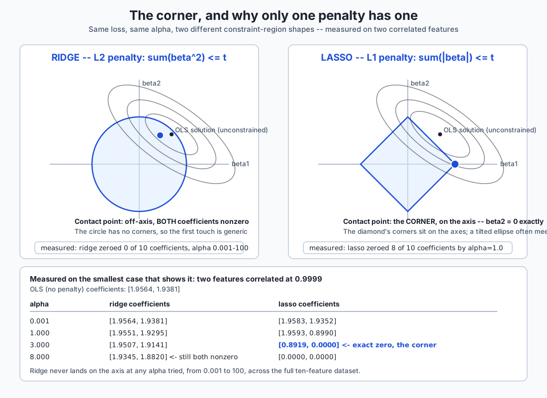
Why the shapes differ: constraint regions and corners
There is an equivalent way to write ridge and lasso that makes the airline analogy exact. Instead of adding a penalty to the loss, imagine minimizing the plain residual sum of squares subject to a hard budget on the coefficients:
ridge, as a constraint:  minimize RSS  subject to  sum_j beta_j^2 <= t
lasso, as a constraint:  minimize RSS  subject to  sum_j |beta_j| <= t
For every alpha there is a matching t, and the two formulations find
the same solution. Picture the unconstrained least-squares solution as a
point in coefficient space, and picture the RSS as a set of nested
elliptical contours around that point — closer to the center means lower
error. The constrained solution is the point where the smallest ellipse
that still touches the feasible region touches it.
Ridge’s feasible region — sum beta_j^2 <= t — is a circle (a sphere
in more than two dimensions). A circle is smooth everywhere; wherever an
ellipse first touches it, that point generically has every coordinate
nonzero, because there is nothing special about the axes from the
circle’s point of view.
Lasso’s feasible region — sum |beta_j| <= t — is a diamond (an
octahedron in more than two dimensions). A diamond has corners, and the
corners sit exactly on the axes. When the loss ellipse is elongated or
tilted relative to the diamond — which is common, especially with
correlated predictors — the first point of contact is very often one of
those corners, and a corner on an axis means one or more coordinates are
exactly zero.
This lesson measured that geometry directly on the smallest case that
still shows it: two features correlated at 0.9999, with an
unregularized (ordinary least squares) solution of [1.9564, 1.9381].
  alpha    ridge coefficients      lasso coefficients
  0.001    [1.9564, 1.9381]        [1.9583, 1.9352]
  0.500    [1.9558, 1.9337]        [1.9588, 1.4176]
  1.000    [1.9551, 1.9295]        [1.9593, 0.8990]
  3.000    [1.9507, 1.9141]        [0.8919, 0.0000]
  8.000    [1.9345, 1.8820]        [0.0000, 0.0000]
At alpha=3.0, lasso’s second coefficient is exactly 0.0 — not
rounded, not small, exactly the corner of the diamond landing on an axis.
Ridge’s second coefficient at the same alpha is 1.9141, and even at
alpha=8.0 — where lasso has zeroed both coefficients completely —
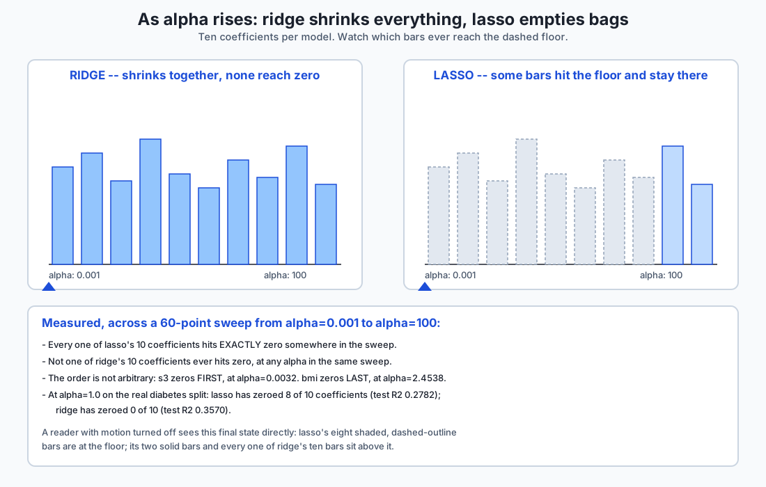
ridge’s are still 1.9345 and 1.8820. Across a much wider sweep, 60
log-spaced alphas from 0.001 to 100 on the full ten-feature diabetes
dataset, every single one of lasso’s ten coefficients hits exactly zero
somewhere in the sweep, and not one of ridge’s ten ever does.
The order coefficients drop in is not arbitrary
The same sweep shows which coefficient zeros first and which zeros last, and the order tracks how much work each feature was doing:
  feature   zeros at alpha =
  s3        0.0032   (first)
  age       0.0126
  s2        0.0126
  s4        0.0495
  s1        0.1597
  s6        0.2360
  sex       0.3487
  bp        1.1242
  s5        2.0188
  bmi       2.4538   (last)
s3 can least afford the fight against the penalty and gives up first.
bmi, which Day 150’s own measurements already flagged as the single
strongest predictor in this dataset, survives longest. Lasso is not
zeroing coefficients in some fixed or alphabetical order — it is zeroing
the ones that contribute least to reducing the residual first, exactly the
way Lasso Air’s passengers would leave the emptiest bag home first.
The gotcha a real measurement caught: alpha is not portable between models
Here is a mistake that is easy to make and expensive to make silently.
Ridge’s objective, as scikit-learn implements it, sums the squared
residuals across every row. ElasticNet’s objective averages them, over
n_samples. So Ridge(alpha=a) is not the same model as
ElasticNet(alpha=a, l1_ratio=0), even though both are pure L2 penalties
in shape — the two alphas live on different scales, off by exactly a
factor of the training-set size.
Measured directly, at n_train = 331: comparing Ridge(alpha=0.1)
against ElasticNet(alpha=0.1, l1_ratio=0.0) without correcting for that
factor gives a test R2 of 0.3690 for ridge and 0.0555 for the
“equivalent” ElasticNet call — a dramatically worse fit, because the
uncorrected ElasticNet call is effectively applying a penalty 331 times
stronger than the ridge call it was supposed to match. Correct for the
factor — fit Ridge(alpha=0.1 * 331) instead — and the two models agree
on their coefficients to within 0.0001:
  Ridge(alpha=0.1 * 331) coefficients[:3]        : [6.3098, 1.2290, 22.6076]
  ElasticNet(alpha=0.1, l1_ratio=0) coefficients[:3] : [6.3097, 1.2290, 22.6076]
This is not a contrived trap. It is exactly the kind of mistake that
happens when someone swaps ElasticNet(l1_ratio=0) in for Ridge
expecting the same tuning to carry over, and it will silently
over-regularize a model with no error message at all. Read the
documentation for whichever library and penalty combination you are
using before you assume two alpha values mean the same thing across two
different model classes.
An everyday analogy
Return to Ridge Air and Lasso Air, and check every measurement above against the story.
Ridge Air’s fee is proportional to weight squared, so nobody arrives
with an empty bag. Measured: ridge zeroed zero of ten coefficients at
every alpha from 0.001 to 1.0, and zero of ten across a 60-point sweep up
to alpha=100. Every bag gets a little lighter as the fee rises; none of
them ever reaches zero.
Lasso Air’s flat per-bag fee makes leaving an under-packed bag at home
the rational move. Measured: lasso zeroed progressively more
coefficients as alpha rose — 0, then 1, then 3, then 8 of 10 — and the
order it zeroed them in tracked exactly how little weight each one was
carrying, s3 first and bmi last.
Two nearly identical suitcases, packed with the same shared cargo.
This is the correlated-predictors case, and it is the clearest place the
two airlines diverge. Picture two bags that are nearly duplicates of each
other — say, a carry-on and a checked bag both stuffed with roughly the
same set of clothes, because you packed in a hurry and did not notice the
overlap. Ridge Air, charging by the square of each bag’s own weight, has
no reason to prefer one bag over the other — it is cheaper to spread the
weight evenly across both than to load either one heavily, so it
splits the cargo close to fifty-fifty. Measured directly on two
predictors correlated at 0.999918, with a true combined coefficient of
6.0: ridge landed on [3.048, 2.9742] at alpha=1.0 — split almost
exactly evenly, and still split almost evenly ([2.9724, 2.9646]) even at
alpha=10.0, ten times stronger. Lasso Air, charging a flat fee per
nonempty bag, has every reason to consolidate: pay the flat fee once, on
one bag, and leave the other one home entirely. Measured: lasso put
5.0848 on one coefficient and drove the other to exactly 0.0 at
alpha=1.0, and at alpha=10.0 it had zeroed both — flat-fee logic
applies even when a bag is genuinely useful, once the fee outweighs what
carrying it is worth.
The airline that weighs your bags in the wrong units. This is the
scale-dependence result, and the analogy makes the mechanism obvious the
moment you say it out loud: imagine Lasso Air’s flat fee is $50 per
nonempty bag, but one gate agent weighs bags in kilograms and another
weighs the exact same bags in grams. A bag holding 2 kilograms reads as
2000 when weighed in grams — a thousand times larger number, for
identical physical cargo — and the flat fee has no way to know the
difference. Whichever bags happen to be measured in the “biggest” numbers
look heaviest to the fee and survive; the ones measured in small numbers
look negligible and get dropped, regardless of what is actually inside
them. That is exactly what raw-units lasso did to the diabetes dataset at
the top of this lesson: it kept all ten features, because in raw
measurement units none of the coefficients looked small enough to be worth
the flat fee of dropping. The penalty was real. It was just being applied
in the wrong units to do anything useful.
Examples in practice
Example 1 — the headline contrast, on
sklearn.datasets.load_diabetes(return_X_y=True) with
train_test_split(test_size=0.25, random_state=0):
| alpha | lasso zeros | lasso test R2 | ridge zeros | ridge test R2 |
|---|---|---|---|---|
| 0.001 | 0/10 | 0.3588 | 0/10 | 0.3586 |
| 0.01 | 1/10 | 0.3541 | 0/10 | 0.3567 |
| 0.1 | 3/10 | 0.3550 | 0/10 | 0.3690 |
| 1.0 | 8/10 | 0.2782 | 0/10 | 0.3570 |
Read the ridge column first, because it is the control: zero zeroed
coefficients, at every alpha tried, full stop. Now read the lasso column:
it climbs steadily. Notice, too, that lasso’s best test R2 in this table
(0.3550, at alpha=0.1) is not far below ridge’s best (0.3690, at the
same alpha) — a sparser model here is not paying a large accuracy
penalty for interpretability, at least not yet, at alpha=0.1. Push
further to alpha=1.0 and lasso’s R2 drops to 0.2782 while ridge’s
recovers to 0.3570 — past a certain point, lasso’s extra sparsity does
start costing real accuracy.
Example 2 — letting cross-validation choose. Hand-picking alpha
from a short list, as the table above does, is a teaching device, not a
real workflow. LassoCV(cv=5) searches a grid automatically and picked
alpha=0.07874 on the training split — a value between the 0.01 and 0.1
rows above — zeroing 4 of 10 coefficients and keeping sex, bmi, bp,
s1, s3 and s5, with a test R2 of 0.3562, competitive with the
hand-picked values.
Example 3 — does lasso recover the right features, not just some
features? The diabetes dataset has no known ground truth — nobody knows
the “true” set of relevant predictors, only what predicts well. To check
recovery honestly, this lesson built a synthetic dataset with
sklearn.datasets.make_regression(n_features=20, n_informative=5), which
returns the exact indices of the five features that actually matter. At
alpha=1.0 and a modest noise level, lasso recovered precision 1.0,
recall 1.0 — the exact five, no more and no fewer. That is a genuinely
strong result and it does not hold unconditionally: push the noise up to
10 or 30 and raise alpha to 80 in the same setup, and recall falls to
0.2 and then to 0.0 — the penalty had become strong enough, on noisy
enough data, to zero out every one of the truly informative features.
Averaged over ten different dataset seeds at a saner alpha=1.0, mean
precision falls from 1.0 at low noise to 0.6792 as noise rises — lasso
starts keeping extra, non-informative features when the signal is harder
to separate from the noise. Regularization is not a one-way ratchet
toward a better model; it is a knob, and it can be turned too far.
Example 4 — the practical scale-dependence result, once more, in
full, all at alpha=1.0 on identical data:
| Units | Features kept | Which ones |
|---|---|---|
| Raw measurement units | 10 of 10 | all ten |
| Standardized (unit variance) | 7 of 10 | sex, bmi, bp, s1, s3, s5, s6 |
scikit-learn’s own scaled=True (unit L2 norm) | 3 of 10 | bmi, bp, s5 |
Notice that even the two “scaled” columns disagree — unit-variance
scaling and unit-norm scaling are both legitimately called “scaled data,”
and they select 7 and 3 features respectively at the identical nominal
alpha. There is no such thing as one universal alpha=1.0; there is
only alpha=1.0 relative to whatever units the coefficients happen to
be in. Standardize your features — sklearn.preprocessing.StandardScaler
is the ordinary choice — before you fit a penalized model, every time,
without exception, and treat any lasso or ridge result fitted on unscaled
inputs as not yet meaningful.
Implications: security, privacy, performance, scalability, and cost
Performance and scalability. Ridge has a closed-form solution — one
linear-algebra call, the same normal-equations machinery Day 149 built by
hand, adjusted by adding alpha to the diagonal before inverting.
Measured directly: a fitted Ridge model carries no n_iter_ attribute
at all, because there was nothing to iterate. Lasso has no closed form,
because the absolute-value penalty is not differentiable at zero, and
scikit-learn solves it by coordinate descent — an iterative algorithm.
Measured iteration counts on the diabetes training split, at
max_iter=50000: 368 iterations at alpha=0.001, 62 at alpha=0.01, 135
at alpha=0.1, and just 6 at alpha=1.0 — heavier penalties converge
faster here, because a strong penalty pushes the solution toward a
simpler, more quickly reached optimum. None of these hit the iteration
ceiling; a Lasso fit that does hit max_iter emits a
ConvergenceWarning and should not be trusted without either raising the
limit or investigating why convergence is slow. At the scale of ten or a
few dozen features, this difference is invisible in wall-clock time. At
thousands of features it becomes a real engineering consideration, and it
is one reason ridge remains the default choice when the goal is purely
predictive accuracy and interpretability is not required.
Security and privacy. A sparser model is a smaller attack and audit surface. A production model that depends on 3 features rather than 10 needs 3 columns of potentially sensitive input at inference time instead of 10, is easier for a reviewer to reason about end to end, and is easier to monitor for drift in the handful of inputs that actually matter. That benefit is only real when the sparsity reflects genuine irrelevance rather than an unscaled penalty accidentally dropping predictive features — which is exactly why the scale-dependence result above is a security-relevant finding and not only an accuracy one. A lasso model fitted on unscaled data and shipped as “the important features” can quietly discard real signal while giving every appearance of principled feature selection.
Cost. Both ridge and lasso are implemented in scikit-learn, which is
free, open source, and requires no account, license, or per-call billing.
The real cost is engineering time: choosing alpha properly means
running cross-validation, which multiplies fitting cost by the number of
folds and the size of the alpha grid searched. LassoCV’s iterative
solve makes that multiplication more expensive than RidgeCV’s
closed-form one, though at the scale used in this lesson — ten features,
a few hundred rows — the difference is a fraction of a second either way.
Alternatives: free, open source, and commercial
scikit-learn — Ridge, Lasso, ElasticNet, and their *CV
variants. Free and open source (BSD 3-Clause). Used throughout this
lesson and its lab. Choose it as the default for anything in Python: the
API is consistent (fit, predict, .coef_), cross-validated variants
handle the alpha search for you, and the closed-form ridge solver and
coordinate-descent lasso solver are both well tested at the scale this
course operates at. Example run in this lesson:
LassoCV(cv=5, random_state=0).fit(X_train, y_train) picked
alpha=0.07874 on the diabetes training split.
statsmodels. Free and open source (BSD 3-Clause). Not installed in
this lab’s environment, so no output from it is reproduced here — it is
described from its public documentation. statsmodels.regression.linear_model.OLS.fit_regularized
offers L1 and a limited elastic-net penalty on top of the classic
statsmodels regression API, which is the natural choice if a project is
already built around statsmodels for its detailed statistical summaries
(standard errors, confidence intervals, hypothesis tests) and needs
regularization added without switching libraries. Its regularization
support is narrower than scikit-learn’s — in particular, cross-validated
alpha selection is not built in the way LassoCV provides it — so most
projects that need heavy hyperparameter search reach for scikit-learn
instead.
glmnet (R, with Python bindings). Free and open source. The original implementation associated with the elastic-net paper, written by Friedman, Hastie and Tibshirani themselves, and still the reference implementation many statisticians reach for first in R. It uses the same coordinate-descent algorithm scikit-learn’s lasso and ElasticNet solvers are built on, and it is described here from documentation only — it was not run for this lesson, since this course’s labs are Python-only. Choose it if your team already works primarily in R, or if you specifically want the reference implementation a published paper’s results were computed with.
Managed AutoML platforms (for example, cloud provider AutoML tabular
services). Paid, usage-based cloud billing — no price is quoted here,
because it varies by provider, region, and workload, and this lesson does
not have a bill to report. These platforms typically include regularized
linear models as one candidate family inside a larger automated search
over several model types, so you get ridge- or lasso-style regularization
as a side effect of a broader hyperparameter search rather than as a
tool you reach for directly. Choose a managed platform when the project’s
constraint is engineering time rather than transparency — you trade
visibility into exactly which penalty and which alpha were chosen for
not having to run that search yourself. This lesson’s lab does not use
one, and no output from any commercial platform is reproduced anywhere in
this content.
Comparison with related concepts
| OLS | Ridge (L2) | Lasso (L1) | ElasticNet | |
|---|---|---|---|---|
| Closed-form solution | Yes | Yes | No | No |
| Ever produces an exact zero coefficient | No | No (measured: never, any alpha) | Yes | Yes |
| Built-in feature selection | No | No | Yes | Yes |
| Handles correlated predictors well | No — unstable, Day 150 | Splits weight evenly (measured) | Picks one, roughly arbitrarily (measured) | Groups them, by design |
| Requires feature scaling | Not for correctness, but recommended | Yes | Yes | Yes |
| Hyperparameters to tune | None | alpha | alpha | alpha, l1_ratio |
Two related ideas worth distinguishing explicitly, since they are sometimes confused with lasso specifically:
Stepwise selection (forward or backward, adding or removing one
feature at a time based on a fit statistic) also produces a sparse final
model, but it is a discrete, greedy search over which features to
include — not a single smooth optimization the way lasso is. It has no
alpha to tune continuously, no coefficient path, and is known to be
statistically unstable: small changes in the data can flip which features
survive the search entirely. Lasso’s selection is a side effect of a
convex optimization problem with well-understood behavior as alpha
varies continuously; stepwise selection’s is not.
Principal component regression (PCR) handles multicollinearity, the same problem ridge was invented for, but by an entirely different route: it transforms the predictors into uncorrelated principal components first, then regresses on a subset of those components. It produces a model with zero coefficients on some components, but those components are linear combinations of the original features, not the original features themselves — so PCR trades away the interpretability that lasso is specifically designed to preserve.
When to use it — and when not to
Reach for ridge when your predictors are correlated (Day 150’s design matrix territory), you want every predictor to remain in the model with a stabilized coefficient, and interpretability in the sense of a short feature list is not the goal — only stable, well-behaved coefficients and solid predictive accuracy are.
Reach for lasso when you have many candidate predictors and want the
model itself to identify a smaller, more interpretable subset as part of
fitting, and you have already scaled your features (non-negotiable — see
the practical result above) and validated alpha by cross-validation
rather than by eye.
Reach for ElasticNet when you have both problems at once: many
candidate predictors, some of which are strongly correlated with each
other, and you want a sparse model that does not arbitrarily discard one
member of a correlated group the way plain lasso measurably does.
l1_ratio gives you a second knob to move continuously between the two
extremes rather than having to commit to one penalty shape outright.
Do not reach for any of the three when you need the model’s coefficients to support a causal or purely explanatory claim about a small, already well-understood set of predictors with little multicollinearity. Regularization deliberately biases coefficients toward zero to buy variance reduction, which is the right trade for prediction but complicates interpreting a coefficient’s magnitude as an unbiased estimate of an effect. Plain OLS, with its unbiased (if higher-variance) coefficients, is the more defensible tool for that narrower job.
Do not reach for lasso specifically when the true structure has several genuinely important, strongly correlated predictors that you want represented together rather than arbitrarily reduced to one survivor — that is precisely the case this lesson measured lasso handling worse than ridge, and it is exactly the case ElasticNet exists to fix.
The AI thread
Weight decay — the L2 penalty applied to a neural network’s weights
during training — is the direct descendant of ridge regression, and it is
turned on by default in the optimizer of essentially every large model
you will train or fine-tune. It shrinks weights toward zero for exactly
the reason ridge does here: it stabilizes an otherwise underdetermined
optimization problem and trades a little bias for a large reduction in
variance, at the scale of billions of parameters rather than ten. What
this lesson’s geometry explains is why weight decay alone does not make a
network sparse — it is an L2 penalty, and L2 penalties do not produce
exact zeros, so a weight-decayed network keeps every parameter, just
smaller. Getting an actually sparse network — for the same reasons lasso
gives you an actually sparse regression, smaller inference cost, a
smaller attack surface, easier auditing — needs an L1-style term or a
dedicated pruning technique layered on top, not weight decay by itself.
The next time you read a training config with weight_decay=0.01 in it,
you are reading alpha from this lesson, doing exactly the job Hoerl and
Kennard described in 1970, at a scale they could not have imagined.
Knowledge check
- At every alpha from 0.001 to 1.0 in the headline table, ridge zeros 0 of 10 coefficients while lasso’s zero count climbs to 8 of 10. Explain in one sentence why the ridge column is the control that makes the lasso column’s climb meaningful.
- Explain, in terms of the constraint-region geometry, why an L1 penalty can produce an exact zero coefficient and an L2 penalty essentially never does.
- On the two-feature demonstration, lasso’s second coefficient is exactly
0.0atalpha=3.0while ridge’s is1.9141at the same alpha. Predict, without recomputing, what ridge’s coefficient would look like atalpha=30instead of3, and explain your reasoning. - The same alpha, on the same data, selects 10, 7, and 3 features depending on whether the data is raw, standardized to unit variance, or scaled to unit L2 norm. What is the one practical rule that follows from this measurement?
Ridge(alpha=0.1)andElasticNet(alpha=0.1, l1_ratio=0.0)are not the same model on the same data. Explain the source of the discrepancy and the correction that resolves it.- On two predictors correlated at 0.999918, ridge splits a true combined
coefficient of 6.0 into roughly
3.05and2.97. What does lasso do to the same two predictors, and why does the airline analogy predict that outcome? - Lasso recovers a known sparse ground truth with precision 1.0 and
recall 1.0 at
alpha=1.0and low noise, but recall falls to 0.0 atalpha=80and high noise. What does that pair of results rule out as a general claim about regularization? - A fitted
Ridgemodel carries non_iter_attribute; a fittedLassomodel always does. What property of the L1 penalty causes that difference, and what would you check on aLassofit that reportedn_iter_equal to itsmax_iter?
Hands-on exercise
Today’s lab, “What the Penalty Does,” measures the ridge-versus-lasso
contrast in eight groups of exercises: the headline zero-count table and
LassoCV’s own alpha choice; the coefficient path and the order
coefficients zero in; whether lasso recovers a known sparse ground truth,
and where that recovery breaks down; the scale-dependence result in full;
ElasticNet and the alpha-scale mismatch with plain ridge; what each
penalty does to near-duplicate predictors; ridge’s closed form against
lasso’s iterative solve; and the smallest case that shows the constraint-
region geometry directly.
Fourteen exercises in total. Build the environment, then work through
starter/test_regularization_claims.py, replacing one pytest.skip at a
time with the assertion its message names.
Expected output
The harness ends with:
---------------------------------------------------------------
14 checks, 0 failure(s)
and exits 0. pytest examples -q reports 18 passed, and
pytest starter -q reports 4 passed, 14 skipped until you begin.
The measured table includes:
   alpha   lasso-zeros   lasso-R2   ridge-zeros   ridge-R2
   0.001       0/10      0.3588        0/10      0.3586
   1.000       8/10      0.2782        0/10      0.3570
  raw                n_kept=10  standardized  n_kept= 7  unit_norm  n_kept= 3
  alpha= 1.000  ridge=[3.048, 2.9742, 0.9944]  lasso=[5.0848, 0.0, 0.0]
Validate your work
bash tests/run_tests.sh; echo "exit=$?"reports14 checks, 0 failure(s)andexit=0. Capture the harness’s own exit status..venv/bin/pytest examples -qreports18 passed..venv/bin/python3 examples/report_measurements.py | diff - expected-output/measured-values.txtproduces no output.- When you have finished every exercise,
pytest starter -qreports18 passed. - Break one assertion on purpose, confirm the harness fails, restore it.
Troubleshooting
import file mismatch. You ran pytest examples starter together.
Both directories define modules with the same names. Run them separately.
ConvergenceWarning from Lasso. The default max_iter=1000 does
not converge on this dataset at small alphas; this lab sets
max_iter=50000 everywhere for exactly that reason. Match it in your own
code.
Your near-duplicate split is not an exact zero. At the default seed
it is ([5.0848, 0.0, 0.0]), but the two columns are correlated at
0.999918, not identically collinear, so other seeds can leave a tiny
nonzero residual instead of a perfect zero. What must hold is a heavily
asymmetric split, not necessarily a bit-exact one.
ElasticNet(l1_ratio=0) does not match Ridge at the “same” alpha.
Expected — see the alpha-scale gotcha above. Correct by multiplying
ridge’s alpha by the training-set size.
Common mistakes
Calling ridge’s shrinkage “feature selection.” Ridge shrinks every coefficient toward zero; it does not reach zero. The headline table’s ridge column, at 0 of 10 zeroed for every alpha tried, is the direct evidence against this.
Fitting lasso on unscaled data and trusting the selected features. The scale-dependence result exists precisely to catch this. Standardize first, always.
Treating “more penalty” as strictly safer. Exercise 3b measures a
case where pushing alpha too high on noisy data drops every one of the
genuinely informative features. Regularization is a knob, not a ratchet.
Requiring an exact zero from lasso at every possible dataset seed. The correlation in the near-duplicate exercise is 0.999918, not 1.0 exactly, so the split can be heavily asymmetric without being bit-exact zero at every seed. Assert the asymmetry, not a floating-point coincidence.
Practice assignment
Take a regression project you already have, or the diabetes dataset used throughout this lesson if you do not, and run the ridge-versus-lasso audit end to end.
- Scale first, and say so. Fit both a ridge and a lasso model on your predictors, standardized. State explicitly which scaler you used and why unscaled data was not an option.
- Sweep
alphaand record the zero count for each model. Confirm that your ridge model’s zero count stays at zero across the whole sweep. If it does not, something in your setup is wrong — recheck it before moving on. - Let cross-validation choose
alphafor you, withLassoCVorRidgeCV, rather than picking a value by eye. Report the chosen alpha and how many features it kept. - Check your predictors for near-duplicates. Compute the pairwise correlation matrix and flag any pair above 0.95. For each flagged pair, report what your lasso model did to it — kept both, split the coefficient, or dropped one — and whether that matches this lesson’s prediction.
- Write one paragraph on which penalty you would ship for this specific project, and why, referencing at least one measured number from your own run rather than a general statement about ridge or lasso.
The deliverable is the audit and the written justification, not a model with a higher score.
Extension challenge
Pick one and measure it.
- Trace the exact path. Use
sklearn.linear_model.lasso_pathto compute the exact piecewise-linear coefficient path scikit-learn derives internally, and compare the alphas it reports each coefficient crossing zero at to the ones this lesson’s grid search found. Report how close the grid-search estimate came. - A three-way tie. Build three near-identical predictors instead of two and measure whether lasso picks exactly one every time, or sometimes splits its selection across two of the three. Report the split rate across several seeds.
- Push the geometry to three dimensions. Extend the two-feature
corner demonstration to three correlated features — an octahedron
against a sphere — and measure how the zero count grows with
alphacompared to the two-feature case. - Reimplement
LassoCV’s search by hand withKFoldand a manual alpha grid, and confirm you recover the same chosen alpha this lesson’sLassoCV(cv=5)call did. - A harder sparse-recovery case. Rebuild the known-ground-truth experiment with correlated informative features instead of independent ones, and measure whether recovery degrades even without adding noise.
- Standardize inside a pipeline. Rebuild the scale-dependence
exercise using
sklearn.pipeline.Pipeline([("scale", StandardScaler()), ("lasso", Lasso(alpha=1.0))])instead of standardizing by hand, and confirm the selected feature set matches.
Quiz
Q1. At every alpha from 0.001 to 1.0 on the diabetes dataset, ridge zeros 0 of 10 coefficients while lasso's zero count climbs to 8 of 10. Why does the ridge column matter to the argument, rather than being a footnote?
- It shows ridge is a worse model, since it never simplifies
- It is the control: holding the data and the alphas fixed and changing only the penalty shape isolates the penalty as the cause of lasso's climbing zero count
- It shows ridge needs a larger alpha to start zeroing coefficients too
- It is not important; only the lasso column is measured in this lesson
Show answer
Answer: B. It is the control: holding the data and the alphas fixed and changing only the penalty shape isolates the penalty as the cause of lasso's climbing zero count
Without the ridge column, lasso's climbing zero count could be explained by almost anything about this particular dataset or fitting procedure. With it, exactly one thing differs between the two columns -- the penalty shape -- and the ridge column staying at zero for every alpha isolates that as the cause. Ridge never zeros a coefficient at any alpha in this lesson's sweeps, including much larger ones than 1.0, so the first option is wrong on the evidence, and the third option invents an alpha where ridge starts zeroing that was never measured.
Q2. Explain why an L1 penalty can produce an exact zero coefficient while an L2 penalty essentially never does, in terms of the constraint region each one defines.
- L1's constraint region is a diamond, with corners sitting on the coordinate axes; L2's is a smooth circle with no corners, so the first point of contact between the loss contours and the region is generically off-axis
- L1 is a stronger penalty than L2 at the same alpha, so it pushes coefficients further toward zero
- L2's constraint region is unbounded, so it can never reach zero, while L1's is bounded
- The difference is a numerical artifact of how scikit-learn's solvers are implemented, not a property of the penalties themselves
Show answer
Answer: A. L1's constraint region is a diamond, with corners sitting on the coordinate axes; L2's is a smooth circle with no corners, so the first point of contact between the loss contours and the region is generically off-axis
The geometric explanation is the one that generalises: a diamond (the L1 feasible region, sum of absolute values <= t) has corners exactly on the axes, and those corners are where one or more coordinates are exactly zero. A circle or sphere (the L2 region) has no such corners, so the point where a loss ellipse first touches it generically has every coordinate nonzero. Neither penalty is simply "stronger" at a given alpha in a way that explains this -- the effect is about shape, not magnitude -- and this lesson measured the geometry directly with real coefficient values, not as a solver artifact.
Q3. The same alpha, on the same diabetes data, selects 10 features in raw units, 7 after standardizing to unit variance, and 3 under scikit-learn's own unit-L2-norm "scaled" convention. What is the one practical rule this measurement establishes?
- Always use scikit-learn's bundled scaled=True version of any dataset, since it gives the sparsest result
- Lasso should never be used on datasets with more than 3 informative features
- A penalty is applied in whatever units the coefficients happen to be in, so features must be scaled -- consistently -- before fitting a regularized model, and even different scaling conventions are not interchangeable at a fixed alpha
- The three results are all equally valid, since they come from the same underlying data
Show answer
Answer: C. A penalty is applied in whatever units the coefficients happen to be in, so features must be scaled -- consistently -- before fitting a regularized model, and even different scaling conventions are not interchangeable at a fixed alpha
The penalty term sums functions of the raw coefficient values, and a coefficient's raw size depends entirely on the units its feature happens to be measured in -- nothing in the fitting procedure corrects for that automatically. The fix is scaling, applied consistently, before fitting. The measurement also shows that "scaled" is not one convention: unit-variance and unit-L2-norm scaling disagree with each other (7 vs 3 features) at the identical nominal alpha, so the first option is wrong to treat one particular scaling as the universally correct choice, and the third option's apparent equivalence is exactly what the measurement rules out.
Q4. Comparing Ridge(alpha=0.1) to ElasticNet(alpha=0.1, l1_ratio=0.0) directly gives R2 0.3690 for ridge and 0.0555 for the "equivalent" ElasticNet call, on identical data. What causes the gap, and what resolves it?
- ElasticNet's coordinate-descent solver has not converged; raising max_iter fixes the gap
- Ridge's objective sums the squared residuals while ElasticNet's averages them over n_samples, so the two alphas are on different scales; fitting Ridge at alpha times n_train instead brings the coefficients into agreement to within 0.0001
- l1_ratio=0.0 is not a valid setting for ElasticNet and silently falls back to a different penalty
- The gap is measurement noise from the random_state used in the train/test split
Show answer
Answer: B. Ridge's objective sums the squared residuals while ElasticNet's averages them over n_samples, so the two alphas are on different scales; fitting Ridge at alpha times n_train instead brings the coefficients into agreement to within 0.0001
This is an alpha-scale mismatch, not a convergence or randomness issue: correcting for the n_train factor (fitting Ridge at alpha * 331 on this split) brought the two models' coefficients to within 0.0001 of each other, confirming the mechanism. l1_ratio=0.0 is a fully valid, well-defined ElasticNet setting -- it just is not automatically the same alpha scale as Ridge's own.
Q5. On two predictors correlated at 0.999918, with a true combined coefficient of 6.0, ridge lands on roughly [3.05, 2.97] at alpha=1.0. What does lasso do to the same two predictors at the same alpha, and why?
- Lasso also splits the weight evenly, since both penalties respond the same way to correlated predictors
- Lasso averages the two predictors into a single new feature before fitting
- Lasso raises an error, since scikit-learn does not permit fitting on collinear features
- Lasso puts nearly the entire combined weight on one predictor (5.0848) and drives the other to exactly 0.0, because a flat per-coefficient cost makes it cheaper to consolidate the weight onto one feature than to pay the cost of keeping both nonzero
Show answer
Answer: D. Lasso puts nearly the entire combined weight on one predictor (5.0848) and drives the other to exactly 0.0, because a flat per-coefficient cost makes it cheaper to consolidate the weight onto one feature than to pay the cost of keeping both nonzero
This is the same shrink-versus-select distinction playing out on correlated predictors specifically: ridge's marginal cost falls as a coefficient shrinks, so splitting the weight is cheap and there is no pressure to consolidate; lasso's marginal cost per nonzero coefficient does not fall the same way, so once a feature's individual contribution is small enough relative to the flat cost of keeping it nonzero, dropping it entirely is the cheaper move. Ridge measurably keeps the split even at ten times the alpha; lasso measurably zeros the second coefficient outright.
Q6. Lasso recovers a known sparse ground truth with precision 1.0 and recall 1.0 at alpha=1.0 and low noise, but recall falls to 0.0 at alpha=80 and high noise -- every informative feature is zeroed. What general claim about regularization does this pair of results rule out?
- That lasso can ever be used for feature selection at all
- That regularization is a one-way improvement -- that more penalty is always at least as safe as less. The measurement shows a heavy enough penalty on noisy enough data can destroy the very signal the selection was supposed to isolate
- That precision and recall are meaningful metrics for a regression problem
- That noise in the data has any effect on which features lasso selects
Show answer
Answer: B. That regularization is a one-way improvement -- that more penalty is always at least as safe as less. The measurement shows a heavy enough penalty on noisy enough data can destroy the very signal the selection was supposed to isolate
The low-noise result already rules out the first option -- lasso recovered the exact truth there. The point of pairing both results is specifically to rule out treating "more regularization" as a strictly safe or monotonically improving choice: at alpha=80 with noise=10, every one of the five truly informative features was zeroed, which is a genuine failure mode, not a smaller version of success. Noise clearly does affect the outcome, which rules out the fourth option directly.
Q7. A fitted Ridge model has no n_iter_ attribute; a fitted Lasso model always does, and its value varies with alpha (368 iterations at alpha=0.001, 6 at alpha=1.0 in this lesson's measurement). What property of the L1 penalty causes this difference?
- Lasso is a more complex model with more parameters to fit than ridge
- The L1 penalty term is not differentiable at zero, so no closed-form solution exists the way ridge's normal equations provide one; scikit-learn instead solves lasso by iterative coordinate descent
- Ridge is only ever fit on small datasets, where an iterative solver would be unnecessary overhead
- n_iter_ is simply not implemented for Ridge in this version of scikit-learn, though it could be added
Show answer
Answer: B. The L1 penalty term is not differentiable at zero, so no closed-form solution exists the way ridge's normal equations provide one; scikit-learn instead solves lasso by iterative coordinate descent
Ridge and lasso fit the same number of coefficients on the same data -- model complexity is not the difference. The absolute-value function in the L1 penalty has a sharp corner at zero where its derivative is undefined, which is exactly what makes the exact-zero solutions possible but also what rules out the same direct linear-algebra solve ridge's smooth, everywhere-differentiable penalty permits. This is a structural fact about the two penalties' shapes, not a version-specific omission or a matter of dataset size.
Q8. Weight decay in a neural-network optimizer is described as ridge regression's direct descendant. Based on what this lesson measured about the L2 penalty, what does weight decay alone NOT do to a network's weights?
- It does not shrink the weights toward zero at all
- It does not stabilize an otherwise poorly conditioned optimization problem
- It does not produce exact zeros -- an L2 penalty shrinks every weight a little without ever driving any of them to be exactly zero, so weight decay alone does not make a network sparse
- It does not apply to the bias terms, only to the weights, which makes it identical to lasso in effect
Show answer
Answer: C. It does not produce exact zeros -- an L2 penalty shrinks every weight a little without ever driving any of them to be exactly zero, so weight decay alone does not make a network sparse
This follows directly from the geometry measured earlier in the lesson: an L2 penalty's smooth, cornerless constraint region means the marginal cost of the last bit of a small coefficient approaches zero, so there is no pressure to reach exactly zero -- confirmed directly by ridge's zero count staying at 0 of 10 across every alpha tested. Weight decay does shrink weights and does help stabilize training, so the first two options are wrong; getting an actually sparse network needs an L1-style term or a dedicated pruning method layered on top, which is the opposite of the fourth option's claim that weight decay alone behaves like lasso.
Glossary
- Regularization
- A term added to a model's training objective that penalizes some measure of complexity -- here, the size of the coefficients -- pushing the fit toward simpler solutions even when a more complex one fits the training data slightly better.
- Ridge regression
- Linear regression with an L2 penalty: the sum of squared residuals plus alpha times the sum of the SQUARED coefficients. Measured here to zero zero of ten coefficients at every alpha tried, from 0.001 to 100.
- Lasso
- Linear regression with an L1 penalty: the sum of squared residuals plus alpha times the sum of the ABSOLUTE VALUES of the coefficients. Measured to zero progressively more coefficients as alpha grows -- 0, then 1, then 3, then 8 of 10 over the same sweep ridge never moved on.
- ElasticNet
- Both penalties combined, with l1_ratio controlling the mix -- l1_ratio=1.0 recovers plain lasso exactly (confirmed here down to the same zero count and R2), l1_ratio=0.0 recovers ridge's penalty shape but NOT its alpha scale.
- Alpha (regularization strength)
- The hyperparameter that scales how much the penalty term matters relative to the residual sum of squares. alpha=0 recovers plain least squares in every model here. Not portable between model classes without correction -- see the Ridge/ElasticNet alpha-scale mismatch.
- Constraint region
- The equivalent way to view a penalty: minimizing the plain loss subject to a hard budget on the coefficients. Ridge's region is a circle (or sphere); lasso's is a diamond (or octahedron), and the diamond's corners, sitting on the coordinate axes, are what makes exact zeros possible.
- Corner solution
- A solution that lands exactly on a corner of the L1 constraint region, meaning one or more coefficients are exactly zero. Measured directly on a two-feature demonstration: lasso's second coefficient equals exactly 0.0 at alpha=3.0, while ridge's is 1.9141 at the same alpha.
- Coefficient path
- Every coefficient's value as alpha is swept from small to large. Lasso's path hits exactly zero for every one of ten features somewhere in a 60-point sweep; ridge's never hits zero at any point in the same sweep. The order lasso's coefficients zero in tracks how much each feature contributes -- the weakest first, the strongest last.
- Sparse ground truth
- A synthetic dataset (built with make_regression) where the exact set of informative features is known in advance, used to measure whether lasso's selection is actually CORRECT rather than merely sparse. Measured precision 1.0 and recall 1.0 at a sensible alpha and low noise; recall 0.0 at a heavy penalty and high noise.
- Scale-dependence
- The fact that a penalty is applied in whatever units the coefficients happen to be in. The single most practically important measurement in this lesson: the identical alpha, on identical data, selected 10, 7 and 3 features under raw, standardized, and scikit-learn's own unit-norm scaling respectively.
- Standardization
- Rescaling each feature to zero mean and unit variance (StandardScaler), the ordinary fix for scale-dependence. Not the same convention scikit-learn's own load_diabetes(scaled=True) uses -- that dataset is unit-L2-norm scaled instead, and the two conventions select different feature sets at the same nominal alpha.
- Feature selection (as a side effect of fitting)
- What lasso does that ridge does not: driving some coefficients to exactly zero as part of a single convex optimization, rather than as a separate discrete search step the way stepwise selection works.
- Coordinate descent
- The iterative algorithm scikit-learn's Lasso and ElasticNet use to find a solution, needed because the L1 penalty is not differentiable at zero and has no closed form. Measured iteration counts on the diabetes split: 368 at alpha=0.001, falling to 6 at alpha=1.0.
- Closed-form solution
- A solution obtained by a single direct calculation rather than an iterative search -- ridge's normal equations, adjusted by adding alpha to the diagonal before inverting. A fitted Ridge model carries no n_iter_ attribute, confirmed here directly, because there was nothing to iterate.
- Weight decay
- The L2 penalty applied to a neural network's weights during training, and ridge regression's direct descendant. Shrinks every weight toward zero but, by the same geometry measured in this lesson, never produces an exact zero -- getting a sparse network needs an L1-style term or pruning on top.
- Grouping effect
- What ElasticNet was designed to restore that plain lasso lacks: treating a group of correlated predictors as a unit, splitting weight among them roughly the way ridge does, rather than picking one arbitrarily and zeroing the rest.
- Near-duplicate predictors
- Two columns correlated at 0.999918 in this lesson's measurement, used to show ridge splitting a true combined coefficient of 6.0 almost evenly (3.048 and 2.9742) while lasso concentrates nearly all of it on one (5.0848) and zeros the other.
- Tikhonov regularization
- The general mathematical technique -- adding a stabilizing penalty term to an ill-posed problem -- introduced by Andrey Tikhonov, of which ridge regression is the linear-regression special case, named and popularized in statistics by Hoerl and Kennard's 1970 paper.
- LassoCV
- Scikit-learn's cross-validated lasso, which searches an alpha grid automatically rather than requiring a value chosen by eye. Measured here to pick alpha=0.07874, zeroing 4 of 10 coefficients and keeping sex, bmi, bp, s1, s3 and s5.
Sources and further reading
- Linear Models -- scikit-learn user guide, Ridge, Lasso and Elastic-Net sections — scikit-learn developers (accessed 2026-08-27)
- Ridge -- scikit-learn API reference — scikit-learn developers (accessed 2026-08-27)
- Lasso -- scikit-learn API reference — scikit-learn developers (accessed 2026-08-27)
- ElasticNet -- scikit-learn API reference — scikit-learn developers (accessed 2026-08-27)
- LassoCV -- scikit-learn API reference — scikit-learn developers (accessed 2026-08-27)
- The Elements of Statistical Learning, chapter 3 on shrinkage methods -- free PDF from the authors — Trevor Hastie, Robert Tibshirani and Jerome Friedman, Springer (accessed 2026-08-27)
- Regularization (mathematics) — Wikipedia (accessed 2026-08-27)
- Lasso (statistics) — Wikipedia (accessed 2026-08-27)
- Tikhonov regularization — Wikipedia (accessed 2026-08-27)
- Regression Shrinkage and Selection via the Lasso (Tibshirani, 1996) -- the original paper, paywalled on JSTOR; the free Elements of Statistical Learning PDF above covers the same method in chapter 3 — Journal of the Royal Statistical Society, Series B, via JSTOR (accessed 2026-08-27)
Kept in this browser, no account needed. Your progress page turns the whole record into one link you can bookmark or open on another device.