Machine Learning › Regression › Day 152
Day 152: Regression Metrics

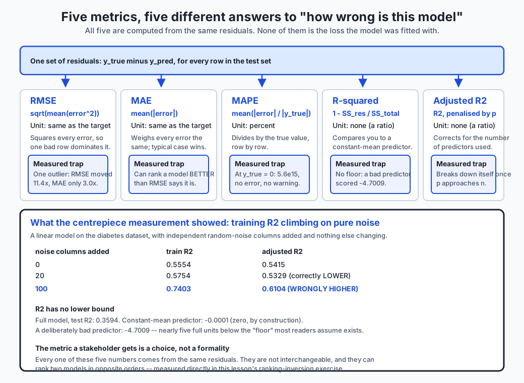
After this lesson you will know why the number you report is a choice, not a formality, because you will have measured a linear model's training R-squared climb from 0.5554 to 0.7403 as you add columns of pure random noise -- columns with exactly zero relationship to the target -- and watched adjusted R-squared correct that climb at a modest predictor count and then break down itself once the predictor count approaches the row count. You will measure that R-squared has no lower bound at all: a deliberately bad predictor scores -4.7009, not the 0 most people assume is a floor. You will move one target value 200 units away from an otherwise unchanged set of predictions and watch RMSE move 11.39 times while MAE moves only 3.00 times, from the same squaring-versus-not-squaring mechanism Day 149 used on the loss side. You will break MAPE at a zero true value and watch it return a number roughly fourteen orders of magnitude too large with no exception and no warning, and you will measure its real structural asymmetry: bounded at 100 percent for the worst possible under-prediction, unbounded for over-prediction. And you will construct two models, scored on the same targets, where RMSE prefers one and MAE prefers the other -- a genuine ranking inversion between the two most common regression metrics, and the single most useful thing in this lesson to carry into a real project.
Hands-on lab for this lesson
Lab files on GitHub: https://github.com/ai-roadmap-365/ai-roadmap-365.github.io/tree/main/labs/sections/machine-learning/day-152-regression-metrics
- Get the hands-on files. Clone the labs repository once (you can reuse this clone for every lesson). This works on macOS, Linux, and Windows (PowerShell or WSL):
git clone https://github.com/ai-roadmap-365/ai-roadmap-365.github.io.git cd ai-roadmap-365.github.io - Open this lesson's lab. Move into the directory for this specific day. Every lab lives at the same predictable path — section / subsection / week / day:
cd labs/sections/machine-learning/day-152-regression-metrics - Read the lab guide. Open `README.md` in that directory. It lists the exact commands, what each does, the expected output, and how to check your work — read it before running anything.
- Run it and check your work. Follow the README's "How to run" section: run the example first to see the finished result, then complete the numbered exercises in `starter/`, then run the tests. The tests pass (exit 0) only when your work is correct.
bash tests/run_tests.sh # or the test command named in the lab README
You can also open the lab as a local page (works offline, shows the file tree and expected output).
Learning objectives
By the end of this lesson you will be able to:
- State the distinction between a loss and a metric precisely, and name which regression metrics this lesson covers
- Demonstrate that a training-set R-squared climbs as predictors are added, even when every added predictor is pure noise
- Compute adjusted R-squared and identify the point at which its own correction breaks down
- State the exact baseline R-squared is measured against, and demonstrate that it has no lower bound
- Explain why RMSE moves more than MAE under a single outlier, in terms of squaring versus not squaring the error
- Construct a true value of zero and a true value near zero and show what each does to MAPE
- State MAPE's real structural asymmetry between over-prediction and under-prediction, and distinguish it from looser folklore claims
- Construct two models where RMSE and MAE disagree about which is better, and explain the mechanism behind the inversion
- State the unit RMSE and MAE are reported in for a real dataset, and explain why a metric without a statable unit cannot be explained to a stakeholder
- Confirm that sklearn.metrics.r2_score agrees with LinearRegression.score, and demonstrate that swapping r2_score's two arguments changes the answer
- Choose which regression metric to report for a stated business question, and defend the choice
- Connect Day 143's classification metric-first lesson (accuracy versus recall) to its regression counterpart measured here
Prerequisites
- Day 149 -- the loss/metric distinction, stated once and handed off explicitly to this day: a loss is what you optimise, a metric is what you report
- Day 143 -- metric-first thinking on the classification side, where accuracy and recall shipped different models on an imbalanced problem
- Day 148 -- the one-predictor linear model and residual plots, which this lesson reports metrics about
- Day 150 -- multiple predictors, which this lesson's noise-column exercise extends directly
- Comfort with NumPy arrays and reading a pytest failure, and a working python3 3.11 or newer on your PATH; the lab builds its own virtual environment and needs no GPU
Why this matters
Add a hundred columns of pure noise to a linear model — numbers with exactly zero relationship to the target, drawn from a random generator that never looks at the data — and watch its training score climb:
  noise columns added   train R2
                    0     0.5554
                    1     0.5555
                    5     0.5648
                   20     0.5754
                  100     0.7403
Every one of those hundred columns is garbage. Not “weak” or “noisy in a useful way” — literally independent random draws, unrelated to the target by construction. And the model’s R-squared, the number most people learn to read as “percent of variance explained,” rose by nineteen points anyway, from 0.5554 to 0.7403.
Nobody cheated. No label leaked. The columns are exactly what they claim to be: noise. What happened is that a training-set R-squared is not a measure of how good a model is. It is a measure of how well the model’s parameters were chosen to fit the exact rows it was shown, and more parameters can always fit those exact rows at least as well as fewer — never worse. This is not a quirk of this dataset. It is a property of ordinary least squares, and it holds for any noise columns, on any data, at any seed.
Here is the second surprise, and it is the one most people have never seen measured. A model can score below zero on R-squared:
  full 10-feature model, test R2       : 0.3594
  constant-mean predictor, test R2     : -0.0001
  deliberately bad (all-zeros), test R2: -4.7009
Most people believe R-squared lives between 0 and 1. Both halves of that belief are wrong. A model can score below zero — a genuinely bad predictor here scored -4.7009, nearly five full units below the floor most people assume exists — and there is no lower limit at all. R-squared does not measure “percent of anything.” It measures one specific comparison: your model’s errors against a baseline that always predicts the mean. Beat that baseline and you are positive. Lose to it — badly — and there is nothing stopping the number from falling as far as your model is bad.
Day 143 already made this kind of point once, on the classification side: a majority-class baseline scored 0.92 accuracy while learning nothing at all, and accuracy and recall shipped two different models on the same imbalanced problem. That was metric-first thinking for classification. Today is the regression counterpart, and it is a genuinely different set of traps — not because regression is harder, but because the metrics themselves behave differently. Accuracy is bounded between 0 and 1 by definition. R-squared is not bounded below at all. RMSE and MAE can rank two models in opposite directions on the same residuals, which this lesson measures directly, in a way that maps exactly onto Day 143’s accuracy-versus-recall inversion but arrives by an entirely different mechanism.
Day 149 drew the line that makes sense of all of this: a loss is what an algorithm optimises while fitting — squared error, in ordinary least squares. A metric is what you report afterward, to someone who was not in the room while the model was being fit, to answer the question “how good is this, really.” Nothing requires the two to be the same function, and today’s whole subject is the reporting side: RMSE, MAE, MAPE, R-squared, and adjusted R-squared — what each one means, what unit it carries, what it hides, and which one is the wrong thing to quote for a given question.
The idea in plain language
Imagine you have finished baking and you want to know how good the cake is. You could weigh how close the finished cake came to the recipe’s exact gram measurements — that is one kind of “how good.” You could ask a panel how it tastes on a percentage scale against the best cake anyone has ever had — that is a different kind. You could ask what percentage of tasters preferred it to a plain, unseasoned version — a third kind again. All three are legitimate answers to “how good is this cake,” and they can disagree, because they are measuring different things.
A regression metric is exactly that kind of choice. You have a model that predicts a number — a price, a duration, a measurement — and a set of actual values it did not get to see while training. There are several honest, standard ways to summarise “how wrong was it, across all those predictions,” and this lesson covers the five that come up constantly: RMSE and MAE, which report the size of the typical mistake in the target’s own units; MAPE, which reports that mistake as a percentage; and R-squared and adjusted R-squared, which report a comparison against a baseline rather than a raw error size.
None of the five is “the correct one.” Each answers a different question, and — this is the part that catches people out — they can disagree about which model is better, on the exact same predictions, for reasons that are not a bug in either metric. Today’s lab constructs two models where this actually happens: one makes many small, consistent mistakes; the other is right almost everywhere and badly wrong a handful of times. RMSE prefers the first. MAE prefers the second. Both preferences are correct, about different things, and picking the metric before you have asked what the business actually needs is picking a winner by accident.
Historical background
Least squares itself is old — Legendre published the method in 1805 and Gauss claimed to have used it since 1795, both fitting astronomical orbit data, and the argument between them over priority is one of the oldest disputes in the history of statistics. But least squares as a loss to optimise and R-squared as a metric to report are historically distinct ideas that arrived separately and got tangled together in how they are taught.
Sir Francis Galton introduced the correlation coefficient in the 1880s while studying how children’s heights related to their parents’ — the same work that gave regression its name, from the “regression toward mediocrity” he observed in heights across generations. Karl Pearson formalised the correlation coefficient mathematically in the 1890s, and R-squared, the square of that correlation in the simple one-predictor case, followed from it directly. R-squared as a general measure of fit for a multiple-regression model — with more than one predictor — was developed and popularised through the early twentieth century, notably in work by Sewall Wright on path analysis in the 1920s, extending correlation-based reasoning to systems of several variables.
The specific problem this lesson opens with — R-squared rising simply because more predictors were added, whether or not they earned their place — was recognised early and named clearly. Henri Theil, writing in the 1960s on regression and forecasting, is generally credited with popularising the adjusted R-squared correction in its modern form, building on earlier degrees-of-freedom corrections that had circulated in statistical practice for decades. The idea is straightforward in principle: penalise R-squared by how many predictors it took to get there, so that adding a useless column no longer looks like an improvement. What this lesson measures — that the correction itself breaks down once the predictor count approaches the row count — is a less commonly taught consequence of the same formula, and it follows directly from how the penalty term is constructed, which the next few sections work through in full.
Mean absolute percentage error has a more recent and more contested history. It became popular in forecasting practice — inventory planning, demand forecasting, economic projections — through the 1970s and 1980s precisely because a percentage is easy to communicate to a non-specialist: “we were off by 8 percent” needs no context about the underlying scale. J. Scott Armstrong, a prominent forecasting researcher, was an early and vocal critic of MAPE’s asymmetry problems in exactly this period, and the debate about MAPE’s flaws versus its communicability has continued in the forecasting literature ever since, including proposals for symmetric variants meant to fix the specific asymmetry this lesson measures directly.
What it is — and what it is not
A regression metric is a summary of the residuals — the differences between what the model predicted and what actually happened — computed after fitting is complete. That is the whole category. Everything below is one specific way of summarising that same list of numbers.
Here is what each of the five metrics in this lesson actually is.
RMSE (root mean squared error) squares every residual, averages the squares, and takes the square root to bring the result back into the target’s own units. Squaring means a large error contributes far more than a small one — an error twice as large contributes four times as much to the sum being averaged.
MAE (mean absolute error) takes the absolute value of every residual and averages it directly. No squaring, so every error contributes to the average in exact proportion to its size — an error twice as large contributes exactly twice as much.
MAPE (mean absolute percentage error) divides each absolute residual by the corresponding true value before averaging, and reports the result as a percentage. It answers “how far off, relative to the size of what we were predicting” rather than “how far off, in absolute terms.”
R-squared compares your model’s total squared error against the total squared error of one specific baseline — a model that ignores every predictor and always guesses the training mean. It reports what fraction of that baseline’s error your model eliminated.
Adjusted R-squared takes R-squared and applies a correction based on how many predictors were used relative to how many rows of data were available, so that adding predictors is no longer free.
Now the things a regression metric is not.
It is not the loss the model was fit with, even when the formula looks identical. Ordinary least squares minimises the sum of squared residuals on the training set while fitting; RMSE as a metric is usually reported on a test set the model never saw. Same arithmetic shape, different data, different purpose — one is what you optimise, the other is what you report, and Day 149 established that distinction is not a technicality.
A training-set metric is not a measure of model quality. This is the
lesson’s opening measurement, restated as a rule: any metric computed on
the same rows a model was fit to will look better than it deserves,
because the fitting process was specifically choosing parameters to make
those exact rows look good. ## Examples in practice below makes the
mechanism concrete for R-squared specifically.
R-squared is not “percent of variance explained” in any sense that guarantees a number between 0 and 1. It is a specific ratio compared against a specific baseline, and that ratio has no floor. The “percent explained” language is a correct intuition only when your model beats the mean-predictor baseline, which is not guaranteed.
No single metric is “the right one.” Each of the five answers a different question about the same residuals, and the next section works through exactly how and why they can disagree.
Why it was created and what problems it solves
Each of these five metrics exists because a specific limitation shows up without it, and each limitation has a measurement in today’s lab.
RMSE and MAE solve the “which errors matter more” question, and they solve it in opposite directions. RMSE, by squaring, treats a few large errors as more important than many small ones. MAE, by not squaring, treats every error as equally important regardless of size. Today’s lab constructs the case where this matters concretely — two models, same targets:
| Model | Error pattern | RMSE | MAE |
|---|---|---|---|
| A | many small, consistent errors | 1.947 | 1.586 |
| B | right on 95 rows, badly wrong on 5 | 4.4353 | 0.8417 |
RMSE says Model A is better. MAE says Model B is better. Both are correct, about different things. RMSE is dominated by Model B’s five bad rows, because each one is squared before it enters the average — a handful of large mistakes can overwhelm a much larger number of small ones. MAE is dominated by the ninety-five rows Model B gets almost exactly right, because nothing is squared and the typical case sets the average. Reporting only one of the two metrics silently picks a winner the other metric disagrees with, and neither number by itself tells you which choice is right — that depends on whether an occasional large error is more costly to whoever uses the model than being typically a little bit off.
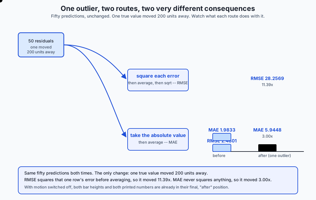
RMSE and MAE also disagree about how much a single outlier should matter, which is the same squaring mechanism from a different angle. Take fifty ordinary predictions, then move one true value 200 units away from the rest without changing any prediction:
  before: RMSE 2.4801  MAE 1.9833
  after : RMSE 28.2569  MAE 5.9448  (one target moved +200)
  RMSE moved by a factor of 11.39
  MAE moved by a factor of 3.00
RMSE moved nearly four times as much as MAE did, on the exact same change to the exact same data. Day 149 measured a version of this on the loss side — how much an outlier distorts the fitted line itself, under squared-error loss versus Huber loss. This is the same mechanism, but the question is different: not “which line gets fit” but “how alarmed should the number you report make you.” An RMSE that jumped 11 times over is not telling you the model got 11 times worse everywhere — it is telling you one row went very wrong, and RMSE is specifically built to shout about that.
MAPE solves the “is this error large or small, relative to what we were predicting” question — and it solves it well only when every true value is safely away from zero. Divide by a true value of exactly zero and here is what actually happens:
MAPE with one true value exactly zero : 5.6295e+15Not an exception. Not a warning. sklearn.metrics. mean_absolute_percentage_error floors the zero denominator at machine
epsilon rather than raising, and the result is a number roughly fourteen
orders of magnitude too large to mean anything — and nothing in the call
signals that it is wrong. A pipeline that logs “MAPE: 5.6e15” without a
human actually reading that line will not catch this. It looks exactly
like a number.
Near-zero true values are almost as bad, without needing an actual zero:
MAPE with a true value of 0.5 in the mix : 3.3667 (MAE on the same rows: 5.0000)MAPE reports 336.67 percent on those three rows. MAE, on the exact same rows, reports a believable 5.0 units of error. One true value is 0.5, and a five-unit miss on a true value of 0.5 is a factor of ten — MAPE reports that honestly, but “336.67 percent error” is not a number most stakeholders can use, even though it is arithmetically correct.
MAPE has a further, structural problem worth being precise about, because the folklore version of this claim is looser than what actually holds. The commonly repeated line is “MAPE penalises over-prediction and under-prediction differently.” Tested directly on equal-magnitude errors applied to a fixed true value — moving a prediction the same absolute distance above and below the truth — MAPE comes out identical in both directions, because its denominator is always the true value regardless of which way the error points. That folklore version does not survive being checked. What does hold, and holds by the metric’s own construction rather than by any property of a particular dataset, is narrower and still important:
  MAPE of the worst possible under-prediction: 1.0000
  MAPE of an eleven-times over-prediction    : 10.0000
The worst possible systematic under-prediction — always guessing zero — cannot score worse than 100 percent MAPE, because the error can never exceed the true value once the prediction floor of zero is reached. Over-prediction has no such ceiling: predicting eleven times the truth scores 1000 percent, and there is no larger multiple that would not score correspondingly larger. Being wrong in one direction is capped. Being wrong in the other is not. That is the real, verified asymmetry — not that equal-size errors are scored unequally, but that the two directions of “very wrong” are not measured on the same scale.
R-squared and adjusted R-squared solve the “compared to what” question. A raw error number — “RMSE was 56” — tells you nothing until you know whether 56 is good or bad for this target’s scale. R-squared answers that by comparing your model against one specific, always-available baseline: guessing the mean. Adjusted R-squared then tries to solve a second-order problem — that R-squared, as the opening measurement showed, climbs mechanically as you add predictors, whether or not those predictors are useful — by penalising the score for how many predictors were used. It works, up to a point, and where that point is is the subject of the next section.
How it works
R-squared, precisely
R-squared compares two quantities: your model’s total squared error, and the total squared error of a model that always predicts the training mean.
R2 = 1 - (sum of (y_true - y_pred)^2) / (sum of (y_true - mean(y_true))^2)The denominator — the mean-predictor’s total squared error — is fixed once you know the data; it does not depend on your model at all. The numerator is your model’s total squared error. If your model’s errors sum to less than the mean-predictor’s, the ratio is less than 1, and R2 is positive: you beat the baseline, and R2 tells you by how large a fraction. If your model’s errors sum to more than the mean-predictor’s — if you did worse than always guessing the average — the ratio exceeds 1, and R2 is negative. There is no floor on how bad the ratio can get, because there is no floor on how bad your model’s total squared error can be relative to the baseline’s.
This is exactly what today’s lab measures directly:
  full 10-feature model, test R2       : 0.3594
  constant-mean predictor, test R2     : -0.0001
  deliberately bad (all-zeros), test R2: -4.7009
The constant-mean predictor scores R2 of essentially exactly zero on fresh test data — not by luck, but by construction, because R2 is defined relative to exactly that predictor. It is the reference point, not an incidental fact about this dataset. And the deliberately bad all-zeros predictor — a genuinely useless model on a target running 25 to 346 — scores -4.7009, which is what “much worse than guessing the mean” looks like on this scale.
Why training R2 climbs on noise, precisely
Ordinary least squares picks the coefficients that minimise the sum of squared residuals on the exact rows it is fit to. Adding a predictor column — any column, including one that is pure noise — gives the fitting procedure one more coefficient to adjust. The old solution, which simply set that new coefficient to zero and ignored the column, is still reachable. So the best the fitting procedure can find with the extra column is at least as good as the best it could find without it, on the training data specifically. It can never be worse.
That is the whole mechanism, and it is a guarantee, not a tendency:
  n_noise   n_rows   n_predictors   train_r2   adjusted_r2
        0      331             10   0.5554     0.5415
        1      331             11   0.5555     0.5402
        5      331             15   0.5648     0.5441
       20      331             30   0.5754     0.5329
      100      331            110   0.7403     0.6104
The train_r2 column is strictly increasing, at every step, on columns
that carry no relationship to the target whatsoever. This is why a
training-set score can never, by itself, be evidence a model has
improved — it is guaranteed to look at least as good with more
predictors, whether or not any of them earned their place.
Adjusted R2, and where its correction breaks down
Adjusted R2 penalises R2 by a factor that grows with the number of
predictors p relative to the number of rows n:
adjusted_R2 = 1 - (1 - R2) * (n - 1) / (n - p - 1)Look at the adjusted_r2 column above and it does exactly what it is
built to do, at first: going from 0 to 20 noise columns, adjusted R2
falls, from 0.5415 to 0.5329, correctly reporting that those twenty
columns did not earn their place even though plain R2 rose. That is the
correction working.
Then look at 100 noise columns. Adjusted R2 is 0.6104 — higher than the 0.5415 baseline, and higher than the 0.5329 it reported at 20 columns — even though every one of those hundred columns is still exactly the same kind of useless noise. The correction has broken down.
The mechanism is visible directly in the formula. At 100 noise columns,
p is 110 (the ten real features plus the hundred noise columns) and n
is 331 training rows — a third of the available data has been spent on
predictors. The term (n - 1) / (n - p - 1) is 330 / 220, about 1.5,
which is a large multiplier on (1 - R2). As p climbs toward n, this
denominator shrinks toward zero and the whole penalty term explodes,
becoming numerically unstable in a way that can push adjusted R2 in
either direction — including, as measured here, back above where it
started. The correction is not a cure for the climb it was built to
catch; it has its own failure mode, and that failure mode is exactly
where you would most want the correction to still be working: many
predictors, not much data.
The practical rule that follows is not “never trust adjusted R2.” It is
“adjusted R2 is trustworthy only while p stays a small fraction of
n,” and once a model has as many predictors as it has rows-to-spare,
no automatic correction — this one included — substitutes for actually
counting how many predictors you have relative to how much data.
RMSE and MAE, precisely
RMSE = sqrt(mean((y_true - y_pred)^2))
MAE  = mean(|y_true - y_pred|)
Both are in the target’s own units, because both undo whatever transformation they applied — RMSE takes a square root to cancel the squaring, and MAE never squares in the first place. This is worth dwelling on because it is the practical reason to prefer either of these over a percentage-based metric when you can: a stakeholder who knows the target’s scale can immediately judge whether an RMSE of 56 is good or bad, because 56 is a number in a unit they already understand.
The one mathematical fact worth having memorised: RMSE is never smaller than MAE, for any set of residuals, with equality only when every residual has exactly the same magnitude. This follows from a standard inequality between the quadratic mean and the arithmetic mean of a set of non-negative numbers. It means an RMSE substantially larger than MAE on the same data is itself informative — it tells you the residuals are not uniform in size, that some rows are much worse than others, before you have looked at a single one.
MAPE, precisely, and where it fails
MAPE = mean(|y_true - y_pred| / |y_true|) * 100The failure mode is visible directly in the formula: y_true is in the
denominator. When y_true is zero, this is a division by zero. When
y_true is small, the ratio is large even for a modest absolute error.
scikit-learn’s implementation does not raise on the zero case — it floors
the denominator at machine epsilon, which produces a large finite number
rather than an error, which is arguably the more dangerous choice, because
a caller who is not specifically checking for it will not notice.
The structural asymmetry follows from the same formula, applied to the
achievable range of predictions rather than to any specific dataset.
Assume predictions cannot go below zero, which holds for most real
targets — a price, a duration, a count. The largest possible
under-prediction is predicting zero, whatever the true value, which gives
|y_true - 0| / |y_true| — exactly 1, or 100 percent, regardless of how
large y_true is. There is no way to under-predict worse than that. But
over-prediction has no matching ceiling: predicting ten times the truth
gives 900 percent; predicting a hundred times the truth gives 9900
percent; the ratio grows without bound as the prediction grows. The
metric’s own denominator guarantees this asymmetry — it is not a property
of any particular dataset, it is a property of the formula.
An everyday analogy
A tailor measuring how well a suit fits.
RMSE is the tailor who is especially bothered by one badly-fitting seam. Ten small adjustments needed across the jacket barely register, but one sleeve two inches too short dominates the tailor’s whole assessment of the fit — squaring the size of each gap, the way RMSE squares each residual, means the one large gap counts disproportionately more than all the small ones combined.
MAE is the tailor who tallies every adjustment equally, however large or small. Ten small nudges and one large one contribute in exact proportion to their size, no more, no less — nothing about a mistake’s size is amplified beyond what it actually is.
MAPE is the tailor who reports every gap as a percentage of the garment part it is on — “the collar is off by 3 percent, the sleeve by 40 percent” — which is genuinely more informative when comparing a large garment part to a small one, until a garment part shrinks toward nothing. Report a gap as a percentage of a buttonhole and a millimetre of error becomes “50 percent off,” a number that is technically correct and practically useless — the same collapse MAPE has near a true value of zero.
R-squared is a tailor who does not report raw measurements at all, but only how much better the fit is than an off-the-rack suit bought without any measurements taken — a “baseline” suit that assumes an average build. If the tailored suit fits far better than that baseline, the score is strongly positive. If, somehow, the tailoring is worse than just grabbing an average-sized suit off the rack — a real possibility if the tailor guessed badly — the score goes negative, and there is no floor on how negative a genuinely bad guess can score.
Adjusted R-squared is the same tailor, except now docked a little credit for every extra measurement taken, on the reasoning that more measurements should only help if they are used well. Take twenty sensible measurements and use them well, and the deduction is small relative to the improvement. Take a hundred pointless measurements — the customer’s shoe size, their favourite colour, their commute time — and even though nothing about the fit could possibly have gotten worse from knowing them, the deduction eventually stops keeping pace: once nearly as many measurements have been taken as there are customers being measured, the correction itself starts behaving strangely, exactly as it did in today’s numbers at 100 noise columns on 331 rows.
Examples in practice
Reading a training R2 versus a test R2
The single most common mistake this lesson exists to prevent: reporting an R2 computed on the same rows a model was fit to, as if it were a measure of how the model will perform on new data.
from sklearn.linear_model import LinearRegression
from sklearn.metrics import r2_score

model = LinearRegression().fit(X_train, y_train)

train_r2 = r2_score(y_train, model.predict(X_train))  # optimistic, guaranteed
test_r2 = r2_score(y_test, model.predict(X_test))      # the honest number
On today’s dataset, train_r2 is 0.5554 with no extra columns and climbs
mechanically as garbage columns are added. test_r2 is 0.3594 and does
not climb with garbage columns, because a test set was never involved in
choosing the coefficients that fit it. Any time a project reports “our
model’s R2 is X” without saying whether X came from training or test
data, the number is not trustworthy on its face — Day 144 covered exactly
why a held-out set is the only honest source for a number like this, and
today’s measurement is the R2-specific version of that same argument.
Choosing between RMSE and MAE for a real decision
An engineer is comparing two models for predicting delivery times. Model A is consistently a few minutes off on every delivery. Model B is almost always right to the minute, but roughly once a week predicts an arrival hours early or late because of an edge case in its logic.
RMSE will report Model B as substantially worse, because that handful of hour-scale misses dominates the squared-error sum. MAE will report Model B as substantially better, because the vast majority of its predictions are excellent.
Which metric to trust depends on what the business does with a bad prediction. If a customer who is told “arriving in 10 minutes” and instead waits three hours will churn regardless of how rare that is, RMSE’s alarm about Model B is the one to listen to. If the business already tolerates occasional bad predictions and cares most about the typical experience, MAE’s preference for Model B is the more useful number. Neither metric is “wrong” — the mistake would be picking one without asking this question first.
Reporting a metric with its unit, or admitting there isn’t one
from sklearn.metrics import mean_squared_error, mean_absolute_error
import numpy as np

rmse = float(np.sqrt(mean_squared_error(y_test, pred)))  # 56.3929
mae = float(mean_absolute_error(y_test, pred))            # 45.1206
A number without a stated unit is not yet a finished report. On the diabetes dataset used throughout this lesson, the target is described in scikit-learn’s own documentation as “a quantitative measure of disease progression one year after baseline” — a composite index running from 25 to 346, with no physical unit such as milligrams per decilitre attached to it. The honest thing to say about an MAE of 45.12 on this target is “the model’s typical prediction is off by about 45 points on a scale that runs from 25 to 346” — not a fabricated real-world unit the dataset’s own documentation does not provide. On a target that does have a real unit — dollars, seconds, kilograms — state that unit explicitly. A metric you cannot state a unit for is a metric you have not finished explaining.
The r2_score argument-order bug
from sklearn.metrics import r2_score

r2_score(y_test, pred)   # 0.359409 -- correct order
r2_score(pred, y_test)   # -0.209635 -- arguments swapped
This looks like a typo that could not possibly matter, and it matters a
great deal. r2_score’s denominator is the variance of whichever array
is treated as “true” — whichever one is passed first — so swapping the
two arguments computes a genuinely different quantity, not the same
quantity read backwards. On this exact data, the correct call reports a
usable model; the swapped call reports a model worse than guessing the
mean, for the identical predictions. The defence is not “be careful” —
that fails eventually on any team. It is to prefer keyword arguments
(r2_score(y_true=y_test, y_pred=pred)) wherever the order is not obvious
from the call site, and to cross-check a computed R2 against a second,
independent source — model.score(X_test, y_test) agrees with the
correctly-ordered call to six decimal places on this data, which is
exactly the kind of independent check that would have caught the swap.
Implications: security, privacy, performance, scalability, and cost
A metric reported without its context is a number that invites misuse. “Our model has an R2 of 0.85” means nothing without knowing whether it is training or test R2, and “our MAPE is 8 percent” means nothing without knowing whether any target value was close to zero. Both omissions are common in real reporting, and both can make a genuinely mediocre model look production-ready to a reader who trusts the headline number.
The argument-order bug in r2_score is a specific instance of a
general class of security- and correctness-relevant mistakes: a
function call that succeeds, returns a plausible-looking value, and is
wrong because two arguments were passed in the wrong positions. The same
shape appears in access-control checks called as (resource, subject)
instead of (subject, resource), in comparison functions, and in
signature-verification calls. The defence — keyword arguments where order
is not obvious, and a second independent check — transfers directly.
Choosing the wrong metric has a cost that shows up only after deployment. A model selected because it minimised MAE, deployed into a context where occasional large errors are unacceptable — a dosage calculation, a structural-load estimate — has been optimised for the wrong failure mode, and the mismatch will not appear in offline testing if the same metric is used for both selection and reporting. This is purely a cost of asking the wrong question early, and it is free to avoid: compute both RMSE and MAE, always, and decide which one governs the decision before comparing models, not after.
MAPE’s silent failure at a zero or near-zero true value is an operational risk in any automated pipeline that logs it unattended. A model-monitoring system that alerts on “MAPE exceeded threshold” will either fire constant false alarms on a target that legitimately passes through zero (returns, refunds, net positions) or, worse, silently report an enormous, meaningless number that a dashboard displays without comment. Either failure is avoidable by checking for near-zero true values before computing MAPE, or by preferring MAE or a scaled error metric on any target that can be zero or near it.
Computing five metrics instead of one costs nothing meaningful. Every metric in this lesson is a single pass over the same array of residuals — on a laptop-scale problem, computing all five takes milliseconds. There is no performance argument for reporting only one; the only reason to report only one is a deliberate decision about what the audience needs to see, which should be a communication choice, not a computational shortcut.
Alternatives: free, open source, and commercial
scikit-learn’s sklearn.metrics — used here
When to choose it: for essentially all in-memory regression work. Free, BSD-3-Clause licensed, no paid tier. Every measurement in this lesson uses it directly.
How to use it: every metric function takes (y_true, y_pred) in that
order and returns a float:
from sklearn.metrics import (
    mean_squared_error,
    mean_absolute_error,
    mean_absolute_percentage_error,
    r2_score,
)

rmse = mean_squared_error(y_true, y_pred, squared=False)  # or sqrt() the MSE
mae = mean_absolute_error(y_true, y_pred)
mape = mean_absolute_percentage_error(y_true, y_pred)
r2 = r2_score(y_true, y_pred)
Watch for: the argument order matters for r2_score and every other
function here, as measured directly above. There is no built-in
adjusted_r2_score in scikit-learn as of this writing — it must be
computed from r2_score, n and p by hand, exactly as this lesson’s
lab does.
statsmodels — described, not run here
When to choose it: for classical statistical regression output — p-values, confidence intervals on coefficients, and adjusted R-squared reported automatically as part of a model summary — rather than scikit-learn’s prediction-first API. Free, BSD-3-Clause licensed.
What it costs: nothing financially; the cost is a different mental
model from scikit-learn’s .fit()/.predict() pattern, closer to R’s
formula-based regression syntax.
Honest note: statsmodels is not installed in this lesson’s lab environment, and no output from it is reproduced anywhere in this lesson. It is described here from its public documentation because it is the standard free tool for a report that needs coefficient-level statistical inference alongside the model-level metrics this lesson covers.
Symmetric MAPE and other MAPE variants — described, not run here
When to choose them: when MAPE’s specific failure modes measured in this lesson — the zero-denominator explosion and the asymmetry between over- and under-prediction — make it unsuitable, but a percentage-style metric is still wanted for communication reasons. Symmetric MAPE (sMAPE) divides by the average of the true and predicted values instead of the true value alone, which softens but does not eliminate the near-zero problem.
What it costs: nothing financially — it is a small amount of extra code, not a paid tool. It is not implemented or measured in today’s lab; extension exercise 4 in the lab asks you to build it and test it against this lesson’s own near-zero construction.
Commercial ML platforms with built-in metric dashboards — not used here
Managed platforms — the kind that log every experiment and compute a standard slate of metrics automatically — remove the risk of a reporting mistake like the ones measured in this lesson, by construction, because the same code path computes every model’s metrics the same way every time. Free versus paid: most offer a free tier for individual use and charge for team features; no price is quoted here, because these change by month and an unchecked figure is worse than none. Open-source self-hosted experiment-tracking tools exist and do the same core job.
Comparison with related concepts
| Metric | What it reports | Unit | Bounded? |
|---|---|---|---|
| RMSE | typical error, large errors weighted heavily | target’s own units | 0 and above, no ceiling |
| MAE | typical error, every error weighted equally | target’s own units | 0 and above, no ceiling |
| MAPE | typical error as a percentage of the true value | percent | 0 and above, no ceiling; explodes near zero |
| R-squared | fraction of the mean-baseline’s error eliminated | none (a ratio) | no floor; ceiling of 1.0 only for a perfect fit |
| Adjusted R-squared | R-squared, penalised for predictor count | none (a ratio) | no floor; loses reliability as predictors approach rows |
Two rows deserve a closing note.
RMSE and MAE never disagree about the direction of a change — if every residual shrinks, both fall; if every residual grows, both rise. They disagree only about magnitude of preference between two different error distributions, which is exactly the ranking-inversion case measured in this lesson. That distinction — same direction, different ranking — is worth holding onto, because it means the disagreement is not a contradiction, it is two different, valid weightings of the same facts.
R-squared and adjusted R-squared are the odd ones out in this table, because they are the only two metrics here defined relative to a baseline rather than as a raw error size. This is precisely why they have no natural unit — a ratio does not carry the target’s units the way RMSE and MAE do — and precisely why R-squared can be negative in a way RMSE and MAE, which are sums of non-negative quantities, cannot.
When to use it — and when not to
Report RMSE when large errors are disproportionately costly, and say so explicitly when you do — a reader who does not know RMSE weighs large errors more heavily may not realise a high RMSE with a modest MAE is telling them something specific about the shape of the errors, not just their average size.
Report MAE when the typical case is what matters, and especially when you want a number a non-technical stakeholder can sanity-check against their own intuition for “how far off is typical” — MAE’s lack of squaring makes it the more directly interpretable of the two for that purpose.
Consider MAPE only when every true value is safely away from zero, and check that condition explicitly before computing it, rather than after seeing a suspicious number. If the target can legitimately be zero or near it — a returns count, a net position, a temperature in Celsius crossing zero — MAPE is the wrong metric regardless of how well the model performs, because the metric itself is what breaks, not the model.
Report R-squared to communicate “how much better than a naive baseline,” and always alongside a raw error metric — RMSE or MAE — because R-squared alone cannot tell a reader the actual scale of the mistakes, only the fraction of a baseline’s error eliminated.
Use adjusted R-squared to compare models with different numbers of predictors on the same data, and stop trusting it once the predictor count becomes a meaningful fraction of the row count — today’s measurement puts that failure mode at p/n around one-third, and the honest response at that point is not a better-corrected R-squared, it is fewer predictors or more data.
Never report a training-set metric as if it were a test-set metric. This is the single rule in this lesson worth memorising above all the others, because the mechanism behind it — more predictors can only help a training-set fit — makes a training metric mechanically optimistic in a way no amount of care in reading it can undo. Only a metric computed on data the model did not influence tells you anything about how it will perform on data it has not yet seen.
The AI thread
Every claim in this lesson gets harder to check, not easier, once the model doing the predicting is a large language model rather than a linear regression.
The metric is often computed by the model itself, or by a system the model has influence over, which turns the argument-order bug and the training-versus-test confusion from careless mistakes into potential incentives. A system that is evaluated on a metric it can also affect — through what it reports, what it selects to show a user, or what training signal it produces for the next iteration — has a structural reason to prefer whichever number looks best, not necessarily whichever number is honest. The discipline this lesson asks for on a small linear model — state the metric, state whether it is train or test, state the unit, cross-check against a second computation — becomes considerably more important, not less, when the system being measured has more surface area to get any one of those steps subtly wrong.
“Percent improvement” claims about model quality inherit every trap this lesson measured, at a scale where nobody re-derives them. A vendor or a paper reporting “R2 improved by 12 percent” is making a claim that depends entirely on whether that R2 was measured on held-out data, how many predictors or features were involved, and what baseline the percentage is relative to — exactly the questions this lesson asks of a diabetes-dataset linear model, unanswered at the scale of a headline benchmark result. The habit worth carrying forward is not suspicion for its own sake — it is the concrete question this lesson practised asking eight times over: what, precisely, is this number being compared against, and on what data was it computed?
And the ranking-inversion measurement generalises directly to model selection at any scale. Choosing between two candidate systems on a single aggregate metric — one number, no breakdown — is exactly the mistake this lesson’s centrepiece exercise was built to make visible: RMSE and MAE disagreed about which of two small linear models was better, for reasons that were real and explainable rather than a bug in either metric. The same disagreement, unexamined, is easy to hide inside a single leaderboard score for a much larger system, where “better on average” can mean “worse on the cases that matter most” without anyone having chosen that trade-off on purpose.
Knowledge check
- A linear model’s training R-squared rises from 0.5554 to 0.7403 as 100 columns of pure random noise are added. Explain the mechanism, and state whether this is evidence the model improved.
- Adjusted R-squared falls to 0.5329 at 20 noise columns but rises to 0.6104 at 100, on 331 rows. Explain both directions of that result.
- A deliberately bad predictor scores R-squared of -4.7009. State precisely what R-squared is being compared against, and explain why there is no lower bound.
- One target value is moved 200 units away from an otherwise unchanged set of fifty predictions. RMSE moves 11.39 times; MAE moves 3.00 times. Explain the mechanism behind the difference in magnitude.
mean_absolute_percentage_erroris called with one true value of exactly zero. State exactly what happens — not what “should” happen — and explain why that specific behaviour is more dangerous than a raised exception.- Two models are scored on the same 100 targets: Model A has RMSE 1.947 and MAE 1.586; Model B has RMSE 4.4353 and MAE 0.8417. Which model is better, and what additional information would you need to answer that with confidence?
- RMSE and MAE are identical whether a linear model is fit on raw-unit or standardised diabetes features. Explain why, and state what unit the resulting numbers are actually in.
r2_score(y_test, pred)andr2_score(pred, y_test)return different values on the same two arrays. Explain the mechanism, and state the defence that would have caught it before it shipped.
Hands-on exercise
Today’s lab, What You Report Is Not What You Optimise, measures every
claim above directly against the diabetes dataset and constructed
examples where a property needs to be exact rather than merely typical.
Twelve exercises. The first two build the noise-column climb and the
adjusted-R2 breakdown. The next two measure R-squared’s missing floor.
Exercises 3 through 5 measure RMSE-versus-MAE under an outlier and MAPE’s
three failure modes. Exercise 6 builds the ranking-inversion pair
directly. The last measure units and the r2_score argument-order bug.
Build the environment, then work through
starter/test_metrics_claims.py, replacing one pytest.skip at a time.
Expected output
The harness ends with:
---------------------------------------------------------------
14 checks, 0 failure(s)
and exits 0. pytest examples -q reports 16 passed, and
pytest starter -q reports 4 passed, 12 skipped until you begin.
The measured table includes:
     n_noise   n_rows   n_predictors   train_r2   adjusted_r2
           0      331             10   0.5554     0.5415
         100      331            110   0.7403     0.6104
  full-model test R2: 0.3594   bad-predictor test R2: -4.7009
  RMSE moved 11.39x, MAE moved 3.00x, under one outlier
  Model A: RMSE 1.947 MAE 1.586   Model B: RMSE 4.4353 MAE 0.8417
Validate your work
bash tests/run_tests.sh; echo "exit=$?"reports14 checks, 0 failure(s)andexit=0. Capture the harness’s own exit status..venv/bin/pytest examples -qreports16 passed..venv/bin/python3 examples/report_measurements.py | diff - expected-output/measured-values.txtproduces no output.- When you have finished every exercise,
pytest starter -qreports16 passed. - Break one assertion on purpose, confirm the harness fails, restore it.
Troubleshooting
Your MAPE number at zero is astronomically large. Expected, and
asserted. mean_absolute_percentage_error does not raise on a zero true
value; it floors the denominator at machine epsilon.
Your adjusted R2 at 100 noise columns is higher than the baseline. Expected, and asserted. The correction’s own penalty term becomes unstable once the predictor count approaches the row count.
import file mismatch. You ran pytest examples starter together.
Run them separately.
Your metrics are identical whether you fit on raw or scaled diabetes features. Correct, and asserted. Ordinary least squares is invariant to a per-column affine rescaling of its inputs.
Common mistakes
Reporting a training-set metric without saying so. The single most important rule in this lesson: a training metric is mechanically optimistic and tells you nothing about performance on new data.
Treating adjusted R2 as an unconditional fix. It corrects the climb at a modest predictor count and breaks down at a high one — both are measured, and both are the point.
Repeating the loose “MAPE penalises directions unequally” folklore without the narrower, verified claim. Equal-magnitude errors on a fixed true value score identically in either direction; the real asymmetry is structural — bounded under, unbounded over.
Quoting one metric from a ranking-inversion pair without the other. RMSE and MAE disagreeing is not a bug to resolve by picking one and hiding the other; it is information about the shape of the errors.
Practice assignment
Take a regression model you already have, or one from a public dataset, and produce a metrics report that would survive this lesson’s scrutiny.
- Report RMSE, MAE, and R2 together, on held-out data, and state explicitly that it is held-out. State the unit RMSE and MAE are in, or state plainly that the target has no natural unit if that is the case.
- Compute adjusted R2 and state
pandnexplicitly. Ifpis more than roughly a tenth ofn, say so, and treat the adjusted R2 figure with the corresponding suspicion this lesson’s measurement earned. - Decide, before comparing any models, whether RMSE or MAE should govern the decision, based on whether occasional large errors are more costly than typical small ones for this specific use. Write the decision down before computing either number.
- Check whether MAPE is safe to report on this target. If any true value is zero or close to it, say so and report MAE or a scaled alternative instead, rather than a MAPE figure that would explode.
- Cross-check one R2 computation with a second, independent method
—
r2_scoreagainst.score(), or a manual formula against the library function — to catch an argument-order or sign mistake before it ships.
The deliverable is the audit and the report, not a better model.
Extension challenge
Pick one and measure it.
- Find the break-even predictor count. Sweep the number of noise columns between 20 and 100 and find where adjusted R2 stops correctly penalising the climb, on this exact dataset. Report the ratio of predictors to rows at that point.
- Implement and test symmetric MAPE. Build it, run it against this lesson’s near-zero-target construction, and report whether it still explodes, and by how much less than plain MAPE.
- Bootstrap a confidence interval for RMSE. Using Days 117-118’s resampling method, put an interval around the RMSE measured before and after the outlier shift, and report how much the interval widens.
- Repeat the noise-column climb with cross-validated R2 instead of training R2. Does the climb still happen? If not, explain precisely what is different about what is being measured.
- Construct a third model for the ranking-inversion pair that is worse than both Model A and Model B on both RMSE and MAE, and confirm there is no metric under which it wins.
- Find a real public dataset with a target that can be exactly zero, and measure MAPE’s failure on real data rather than a constructed example. Report what a naive pipeline would have logged.
Quiz
Q1. A linear model is fit on the diabetes dataset, then refit with 100 extra columns of independent random noise added -- numbers with exactly zero relationship to the target. Its TRAINING R-squared rises from 0.5554 to 0.7403. What is the correct explanation?
- This indicates a bug in the R-squared calculation, since unrelated columns should not change the score
- More predictors can only reduce or leave unchanged the training sum of squared residuals, because the original fit is always still reachable -- so training R-squared is non-decreasing in the number of predictors, regardless of whether they are useful
- The extra columns happened to be correlated with the target by chance, which is likely with 100 random draws
- The model is using the noise columns to memorise individual rows, the same mechanism as a 1-nearest-neighbour classifier
Show answer
Answer: B. More predictors can only reduce or leave unchanged the training sum of squared residuals, because the original fit is always still reachable -- so training R-squared is non-decreasing in the number of predictors, regardless of whether they are useful
This is a property of ordinary least squares, not an accident of this dataset or these particular noise columns: adding any column, however useless, can only help or leave unchanged a training-set fit, because the fit that ignored the new column entirely (coefficient zero) is still available. Chance correlation contributes to the exact size of the climb but is not the reason it is guaranteed; harness check 8 confirms the climb happens at several further seeds, which chance correlation alone would not guarantee. Nothing about this indicates a bug, and there is no memorisation mechanism in linear regression analogous to 1-NN.
Q2. Adjusted R-squared falls from 0.5415 to 0.5329 when 20 noise columns are added (correctly detecting that they did not help), but RISES to 0.6104 when 100 noise columns are added, on 331 training rows. What does this measure?
- Adjusted R-squared's own correction term becomes unstable once the number of predictors (110) becomes a large fraction of the number of rows (331), so the correction itself breaks down -- it is not an unconditional fix for the climb it was built to catch
- The 100-noise-column model is being scored on a different, larger validation set, which explains the higher number
- A rounding error in how adjusted R-squared was computed at high predictor counts
- Adjusted R-squared corrects for overfitting perfectly at any predictor count, and 0.6104 must reflect a real relationship the model found
Show answer
Answer: A. Adjusted R-squared's own correction term becomes unstable once the number of predictors (110) becomes a large fraction of the number of rows (331), so the correction itself breaks down -- it is not an unconditional fix for the climb it was built to catch
Adjusted R-squared''s formula, 1 minus (1 minus R-squared) times (n-1)/(n-p-1), has a penalty term that grows sharply as p approaches n. At p=110 on n=331 rows that term is large enough to overwhelm the correction and let adjusted R-squared climb back above the baseline, even though every added column is still pure noise. This is a real, measured failure mode of the correction, not a rounding artefact, not evidence of a real relationship, and both figures are computed on the same training set with no validation set involved.
Q3. A deliberately bad predictor (predicting zero for every row) scores an R-squared of -4.7009 on the diabetes test set. What does a negative R-squared mean?
- It is a formula error; R-squared cannot go below zero because it is defined as a percentage of variance explained
- The test set itself is corrupted, since a properly split test set cannot produce a negative score
- The model has negative variance, which is only possible for classification problems misapplied to regression
- R-squared is defined relative to a constant-mean predictor, and a model that performs worse than always guessing the mean scores below zero -- with no lower bound, because there is no limit on how much worse than the mean baseline a bad model can be
Show answer
Answer: D. R-squared is defined relative to a constant-mean predictor, and a model that performs worse than always guessing the mean scores below zero -- with no lower bound, because there is no limit on how much worse than the mean baseline a bad model can be
R-squared is one minus the ratio of your model''s sum of squared errors to a constant-mean predictor''s sum of squared errors. There is no mathematical floor on that ratio: a sufficiently bad model''s error sum can exceed the mean predictor''s by any amount, which is exactly what happened here. This is not a formula error, has nothing to do with classification, and says nothing about test-set corruption -- the constant-mean predictor and the full model on the same split both score as expected (-0.0001 and 0.3594 respectively).
Q4. Fifty predictions are unchanged, but one true value is moved 200 units away from the rest. RMSE moves from 2.4801 to 28.2569 (11.39 times); MAE moves from 1.9833 to 5.9448 (3.00 times). Why does RMSE move so much more?
- RMSE is a biased estimator and MAE is unbiased, which explains the difference
- RMSE squares each error before averaging (and later takes a square root), so one very large error dominates the sum; MAE never squares anything, so the same error contributes only in proportion to its size
- MAE was computed on a smaller sample than RMSE in this measurement, making it less sensitive to the outlier
- RMSE is measured in different units than MAE, so the two numbers are not directly comparable
Show answer
Answer: B. RMSE squares each error before averaging (and later takes a square root), so one very large error dominates the sum; MAE never squares anything, so the same error contributes only in proportion to its size
Squaring a large error produces an enormous contribution to the sum being averaged; absolute value never does. This is the same squaring-versus-not-squaring mechanism Day 149 measured on the LOSS side (which line gets fit), applied here to what gets REPORTED after fitting. RMSE and MAE are both in the target''s own units, computed on the same fifty rows, and neither estimator''s bias is the relevant property here -- the effect is about sensitivity to one large error, not about expected value over repeated samples.
Q5. `mean_absolute_percentage_error` is called with one true value of exactly zero. What actually happens, and why does it matter?
- It automatically excludes that row from the average and computes MAPE over the remaining rows
- It returns NaN with a RuntimeWarning printed to the console, alerting the caller to the problem
- It silently returns a huge, meaningless number -- roughly 5.6e15 on the exact rows this lesson uses -- with no exception and no warning, which is more dangerous than a crash because the value looks like a number a caller might not think to question
- It raises a ZeroDivisionError immediately, which is the correct and safe behaviour
Show answer
Answer: C. It silently returns a huge, meaningless number -- roughly 5.6e15 on the exact rows this lesson uses -- with no exception and no warning, which is more dangerous than a crash because the value looks like a number a caller might not think to question
scikit-learn floors the zero denominator at machine epsilon rather than raising or warning, which produces a finite but enormous, meaningless value. The genuinely important part of this fact is NOT that the value is wrong -- it is that nothing in the call signals it is wrong. A raised exception or a warning would at least alert a caller; a silently returned huge float does not, and a pipeline that logs "MAPE: 5.6e15" without a human reading it will not catch this. No row is excluded, and nothing is printed.
Q6. Two models are scored on the same 100 targets. Model A makes many small, consistent errors: RMSE 1.947, MAE 1.586. Model B is right on 95 rows and badly wrong on 5: RMSE 4.4353, MAE 0.8417. Which model is better?
- Model A, because RMSE is always the more trustworthy metric for model comparison
- Neither model is usable, since a metric disagreement always indicates a bug in at least one of the two evaluations
- The question cannot be answered from the metrics alone -- RMSE and MAE genuinely disagree here, and the correct choice depends on whether occasional large errors are more costly to the business than being typically slightly off, which is a domain question neither metric answers by itself
- Model B, because MAE is always the more trustworthy metric for model comparison
Show answer
Answer: C. The question cannot be answered from the metrics alone -- RMSE and MAE genuinely disagree here, and the correct choice depends on whether occasional large errors are more costly to the business than being typically slightly off, which is a domain question neither metric answers by itself
This is a real ranking inversion, not a bug: RMSE prefers Model A because it is dominated by Model B''s few large misses; MAE prefers Model B because it is dominated by the 95 rows Model B gets almost exactly right. Neither metric is unconditionally "more trustworthy" -- each answers a different question about the same residuals. If occasional large errors are unacceptable (a dosage, a structural load), RMSE''s preference for A is the one to act on; if the typical case matters most and the five bad rows are tolerable, MAE''s preference for B is. A metric disagreement like this is expected behaviour, not evidence of a bug.
Q7. RMSE and MAE are reported as 56.3929 and 45.1206 on the diabetes test set, identically whether the model was fit on raw-unit features (age in years, bmi, raw blood pressure) or on standardised features. What does this identical result demonstrate, and what unit are those two numbers in?
- It demonstrates that the raw and scaled feature sets happen to contain exactly the same information by coincidence in this particular dataset
- It demonstrates that ordinary least squares is invariant to a per-column affine rescaling of its inputs, so the predictions (and every metric computed from them) are identical either way; the numbers are in the diabetes target's own units, which is a composite disease-progression score with no physical unit such as mg/dL
- It demonstrates a bug -- fitting on differently scaled features should change the predictions and therefore the metrics
- It demonstrates that RMSE and MAE are always identical regardless of what units the TARGET itself is measured in
Show answer
Answer: B. It demonstrates that ordinary least squares is invariant to a per-column affine rescaling of its inputs, so the predictions (and every metric computed from them) are identical either way; the numbers are in the diabetes target's own units, which is a composite disease-progression score with no physical unit such as mg/dL
Rescaling a predictor column by an affine transform (mean-centring and dividing by a constant, as standardisation does) does not change what ordinary least squares can express, so the fitted predictions -- and every metric computed from them -- are identical. This is a property of the estimator, not a coincidence of this dataset. RMSE and MAE ARE affected by the target''s own units (a metric on a target measured in dollars looks different from the same relationship measured in cents); what does not affect them is the units of the FEATURES. The diabetes target itself has no physical unit -- inventing one, such as mg/dL, would be a fabrication the dataset''s own documentation does not support.
Q8. `r2_score(y_test, pred)` returns 0.359409. Calling it with the arguments swapped, `r2_score(pred, y_test)`, returns -0.209635 -- the same predictions now look worse than guessing the mean. What is the correct explanation?
- r2_score always returns a negative number when called with the arguments in the wrong order, regardless of the data
- The swapped call is measuring the model's performance on the training set instead of the test set
- r2_score has a bug that only appears with this particular dataset
- r2_score is not symmetric in its two arguments: its denominator is the variance of whichever array is passed first, so swapping y_true and y_pred computes a genuinely different quantity, not the same quantity read backwards
Show answer
Answer: D. r2_score is not symmetric in its two arguments: its denominator is the variance of whichever array is passed first, so swapping y_true and y_pred computes a genuinely different quantity, not the same quantity read backwards
r2_score''s formula divides by the variance of whichever array is treated as "true", so which array is passed first changes the computation, not merely the presentation of the result. This is not a bug specific to this dataset -- it is documented behaviour that surfaces differently on every pair of non-identical arrays, and the sign of the result on a swap is not universally negative, only whatever the swapped formula happens to produce for a given pair of arrays. Neither call touches the training set; both use the same test-set arrays in different positions.
Glossary
- Loss
- What an algorithm minimises while fitting a model, established on Day 149. Distinct from a metric, which is what you report afterward to judge the result -- the two need not be the same function, and this lesson covers the reporting side.
- Metric
- What you report after fitting, to judge a model's result. RMSE, MAE, MAPE, R-squared and adjusted R-squared are all metrics, and none of them is required to be the function the model was fitted to minimise.
- RMSE
- Root mean squared error -- the square root of the average squared residual. In the target's own units. Squares every error before averaging, so one very wrong prediction dominates it: measured here moving 11.39 times under a single outlier while MAE moved only 3.00 times.
- MAE
- Mean absolute error -- the average of the absolute value of every residual. In the target's own units. Weighs every error equally, so it is dominated by the typical case rather than by a handful of large misses.
- MAPE
- Mean absolute percentage error -- the average of each residual divided by its true value, expressed as a percentage. Undefined at a true value of zero; scikit-learn does not raise or warn there, it floors the denominator at machine epsilon and returns a huge, silently wrong number -- measured here at roughly 5.6e15.
- R-squared
- One minus the ratio of a model's sum of squared errors to a constant-mean predictor's sum of squared errors. Not bounded below by zero: a deliberately bad predictor measured here scored -4.7009. Dimensionless, unlike RMSE and MAE.
- Adjusted R-squared
- R-squared penalised by the number of predictors used relative to the number of rows. Corrects the training-R2 climb at a modest predictor count -- measured falling from 0.5415 to 0.5329 at 20 pure noise columns -- but breaks down itself once the predictor count approaches the row count, measured climbing back to 0.6104 at 100 noise columns on 331 rows.
- Constant-mean predictor
- The baseline predictor R-squared is defined relative to -- always guess the training mean. Measured here scoring R-squared of -0.0001 on fresh test data, essentially exactly zero by construction, which is the fact R-squared's zero point actually represents.
- Training R2 climb
- The rise in a model's R-squared measured on the same rows it was fit on, as predictors are added, regardless of whether those predictors carry any real relationship to the target. Measured here at 0.5554 to 0.7403 across 0 to 100 pure-noise columns -- not a sign of a better model, a mechanical consequence of ordinary least squares.
- Metric ranking inversion
- When two metrics disagree about which of two models is better, because each weighs the same residuals differently. Measured here directly: RMSE preferred a model with many small errors, MAE preferred a model with a few large ones -- the regression counterpart of Day 143's accuracy-versus- recall inversion on classification.
- Argument-order bug
- A class of bug where a function's answer depends on which argument occupies which position, and swapping them produces a plausible-looking but wrong answer rather than an error. sklearn.metrics. r2_score is not symmetric in y_true and y_pred; measured here returning 0.359409 in the correct order and -0.209635 swapped.
- Affine-rescaling invariance
- A property of ordinary least squares: fitting on features rescaled by a per-column affine transform (mean-centred and divided by a constant, as standardisation does) produces identical predictions to fitting on the original features. Measured here as identical RMSE, MAE and R2 on raw-unit and standardised diabetes features.
- Unit of a metric
- What RMSE and MAE are stated in -- the same units as the target. A metric you cannot state a unit for is a metric you cannot explain to a stakeholder; the diabetes target itself has no physical unit, being a composite disease-progression score, which this lesson states plainly rather than fabricating one.
- MAPE's structural asymmetry
- The verified, narrow claim about MAPE's directional bias: the worst possible systematic under-prediction (always guessing zero) caps out at 100 percent, while over-prediction has no ceiling -- measured here at 1.0 versus 10.0 for an eleven-times over-prediction. Narrower than the folklore claim that equal-magnitude errors are scored unequally, which does not hold under direct construction.
- Selection of a regression metric
- The decision, made before reporting, about which function best answers the actual business question -- whether occasional large errors are more costly than being typically slightly off, whether a percentage is meaningful given the target's scale, and what unit a stakeholder needs to hear. Not a formality; measured directly to change which of two models looks better.
- Test R2
- R-squared measured on data the model was not fit on -- the honest number, as opposed to training R2, which climbs mechanically as predictors are added. Measured here at 0.3594 for the full ten-feature diabetes model, unaffected by whether the model was fit on raw or standardised features.
Sources and further reading
- Regression metrics -- scikit-learn user guide — scikit-learn developers (accessed 2026-08-27)
- r2_score -- scikit-learn API reference — scikit-learn developers (accessed 2026-08-27)
- mean_absolute_percentage_error -- scikit-learn API reference — scikit-learn developers (accessed 2026-08-27)
- The Diabetes dataset -- scikit-learn toy datasets — scikit-learn developers (accessed 2026-08-27)
- Coefficient of determination (R-squared) — Wikipedia (accessed 2026-08-27)
- Mean absolute percentage error — Wikipedia (accessed 2026-08-27)
- The Elements of Statistical Learning, chapter 7 on model assessment -- free PDF from the authors — Trevor Hastie, Robert Tibshirani and Jerome Friedman, Springer (accessed 2026-08-27)
- Adjusted R-squared — Wikipedia (accessed 2026-08-27)
Kept in this browser, no account needed. Your progress page turns the whole record into one link you can bookmark or open on another device.