Machine Learning › Regression › Day 153
Day 153: Linear Regression from Scratch

After this lesson you will have built ordinary least squares three ways -- the normal equations, an lstsq-based solve, and gradient descent -- and measured exactly what a good library was doing for you that the textbook formula does not. You will watch a design matrix with one near-duplicate column send the normal-equation and lstsq coefficients to plus and minus two hundred thousand while scikit-learn's own LinearRegression stays at 2.5 and 2.5, and you will measure why: cond(X'X) is exactly the square of cond(X), confirmed to ten decimal places on well-conditioned data and measured to degrade under extreme ill-conditioning on the dramatic case. You will apply Day 111's gradient- descent stability condition to a real Hessian's eigenvalues and predict, to the decimal, the learning rate at which convergence turns into divergence -- then measure gradient descent struggling for 200,000 iterations on badly scaled raw features where it converges in thousands on standardized ones. You will count operations rather than time them, and find the closed form needs about a thousand times fewer multiply-adds than gradient descent needs to match it. You will build a scikit-learn-compatible estimator, citing Day 146's measured reason for inheriting BaseEstimator rather than re-deriving the contract, and run the real check_estimator suite against it -- reporting 48 of 52 checks passing and naming the two that do not.
Hands-on lab for this lesson
Lab files on GitHub: https://github.com/ai-roadmap-365/ai-roadmap-365.github.io/tree/main/labs/sections/machine-learning/day-153-linear-regression-from-scratch
- Get the hands-on files. Clone the labs repository once (you can reuse this clone for every lesson). This works on macOS, Linux, and Windows (PowerShell or WSL):
git clone https://github.com/ai-roadmap-365/ai-roadmap-365.github.io.git cd ai-roadmap-365.github.io - Open this lesson's lab. Move into the directory for this specific day. Every lab lives at the same predictable path — section / subsection / week / day:
cd labs/sections/machine-learning/day-153-linear-regression-from-scratch - Read the lab guide. Open `README.md` in that directory. It lists the exact commands, what each does, the expected output, and how to check your work — read it before running anything.
- Run it and check your work. Follow the README's "How to run" section: run the example first to see the finished result, then complete the numbered exercises in `starter/`, then run the tests. The tests pass (exit 0) only when your work is correct.
bash tests/run_tests.sh # or the test command named in the lab README
You can also open the lab as a local page (works offline, shows the file tree and expected output).
Learning objectives
By the end of this lesson you will be able to:
- Implement ordinary least squares via the normal equations, an lstsq-based solve, and batch gradient descent, from first principles
- Explain why cond(X'X) is exactly the square of cond(X), and state the textbook consequence for numerical precision
- Construct a design matrix on which the normal equations and lstsq both fail while a library implementation does not, and explain the mechanism
- Apply Day 111's stability condition, |1 - eta * a| < 1, to a measured Hessian's eigenvalues to predict a gradient-descent divergence boundary exactly
- Measure how badly scaled features multiply a Hessian's condition number, and connect the resulting slowdown to Day 111's material rather than treating it as a new fact
- Count the operations a closed-form solve and an iterative method use, and state when each is the right choice as a function of problem shape
- Build a scikit-learn-compatible estimator by inheriting BaseEstimator and RegressorMixin, citing Day 146's measured requirement rather than re-deriving it
- Run sklearn.utils.estimator_checks.check_estimator against a from-scratch estimator and report a real pass/fail count by name, without suppressing failures
- Compare two implementations of fit_intercept -- centring versus an appended column of ones -- and confirm they agree to measured precision
- Distinguish a genuinely singular design matrix from a merely ill-conditioned one, and state why lstsq degrades more gracefully than the normal equations at both
- Recognise multicollinearity, introduced structurally on Day 150, as the same phenomenon this lesson measures numerically at the level of floating-point arithmetic
- Explain, with a measured example, why a library's default solver choice is a numerical-stability decision and not an arbitrary implementation detail
Prerequisites
- Day 111 -- gradient descent, its update rule, learning-rate regimes from |1 - eta a|, and the condition number as the ratio of the Hessian's eigenvalues; none of that is re-derived here
- Day 146 -- the scikit-learn estimator API contract and the measured requirement that a from-scratch estimator inherit BaseEstimator to survive Pipeline.predict() and cross_val_score
- Day 148 -- the one-predictor model and what a fitted coefficient means
- Day 149 -- the loss function and where the normal equations come from
- Day 150 -- many predictors and multicollinearity, which this lesson measures as a numerical-precision problem rather than a purely statistical one
- Comfort with NumPy arrays, matrix multiplication, and reading a pytest failure, and a working python3 3.11 or newer on your PATH; the lab builds its own virtual environment and needs no GPU
Why this matters
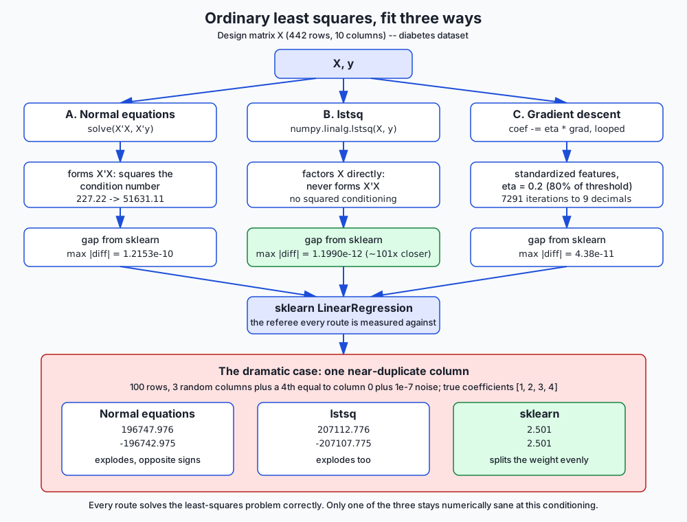
Three random columns of noise. A fourth column that is almost identical to
the first — the same numbers, with a sliver of noise added, 1e-7 in
scale, far below anything a real sensor would ever add. The true
relationship is y = 1*x0 + 2*x1 + 3*x2 + 4*x3, plus a little measurement
noise. Fit it with the textbook formula for linear regression, the one
every statistics course writes on the board:
  true coefficients                : [1, 2, 3, 4]
  normal-equation coefficients     : [196747.976, 1.997, 2.994, -196742.975]
  lstsq coefficients               : [207112.776, 1.997, 2.994, -207107.775]
  sklearn LinearRegression         : [2.501, 2.000, 2.997, 2.501]
Read the first row again. The true weight on that first column is 1. The
textbook formula returns 196,747.976. Not a typo, not a sign error —
a coefficient two hundred thousand times too large, paired with an equally
enormous negative number on the near-duplicate column next to it, so that
the two together still add up to roughly the right prediction. lstsq,
NumPy’s more careful least-squares solver, does no better — it explodes to
207,112.776. Only scikit-learn’s own LinearRegression, given the exact
same data, lands at 2.501 and 2.501: sane, close to the true value split
evenly between the two columns that are nearly saying the same thing.
Nobody made an arithmetic mistake. Every one of these three routes solves the least-squares problem correctly — each finds coefficients that minimize the sum of squared errors on this data, and if you check their predictions against the training data, all three predict almost identically well. The catastrophe is invisible in the predictions and entirely visible in the coefficients. If you were using this model to decide which of four factors mattered most, the textbook formula would tell you factor one matters two hundred thousand times more than anything else in the universe — and it would be measuring nothing but a rounding error dressed up as a huge number.
This is the day Course04 stops calling .fit() and starts asking what
.fit() does. Days 148 through 152 taught you what a fitted coefficient
means, where the formula for it comes from, what happens with many
predictors, how to regularize, and how to measure a model’s quality. Every
one of those days trusted LinearRegression() to return the right
numbers. This lesson builds the fit three separate ways — the normal
equations, an lstsq-based solve, and gradient descent — and measures
precisely where each one agrees with the library, where it does not, and
why. The answer turns out to be a single number, squared, and it connects
directly to Day 150’s multicollinearity and Day 111’s gradient descent,
neither of which is re-taught here — both are about to arrive exactly
where they matter.
The idea in plain language
Imagine you are trying to guess two people’s weights from the weight of the couch they carried up the stairs together. You know the couch weighed 80 kilograms combined. You have no idea how it split between them.
If the two people are clearly different sizes — one visibly twice the other — there is a natural, well-determined split: two-thirds and one-third, say. But if the two people are identical twins, standing shoulder to shoulder, carrying identically, there is no way to determine the split from the couch weight alone. Any split that adds to 80 explains the data equally well: 40 and 40, or 79 and 1, or negative 500 and 580. The data simply does not contain the information to separate them.
That is exactly what a near-duplicate column does to a regression. When two predictors carry almost the same information, the combined effect on the outcome is well-determined — the model can nail the prediction — but the individual coefficients are not. Any pair of numbers that adds up to roughly the right combined effect fits almost equally well, and a solver that is not built to notice this will happily report an absurd pair, like 79 and 1, or 196,747.976 and negative 196,742.975, because nothing in its arithmetic says “prefer the boring answer.”
The textbook formula for linear regression — literally invert a matrix and multiply — has no opinion about which of the infinitely many equally-good splits to report. It reports whichever one the arithmetic of matrix inversion happens to produce, and that arithmetic is unstable exactly when two columns are close to saying the same thing: tiny floating-point rounding errors, ordinarily invisible, get amplified into enormous coefficient swings. A good library’s default solver, by contrast, is built to prefer the boring answer — the smallest, most reasonable split among the many that fit — and that preference is not a statistical choice, it is a numerical one, made for reasons this lesson is about to measure directly.
Historical background
Least squares is one of the oldest working algorithms in applied mathematics. Carl Friedrich Gauss claimed to have used it from 1795, and it was published independently by Adrien-Marie Legendre in 1805, in his work on determining the orbits of comets from imprecise astronomical observations — itself a story about extracting a stable signal from noisy measurements, which is the whole subject of this lesson viewed from a different angle. For a century and a half after that, “solve the normal equations” and “fit a linear regression” were effectively the same sentence, because forming and inverting a small matrix by hand or by mechanical calculator was already hard enough; nobody was worrying about which of two mathematically equivalent formulas lost fewer decimal digits.
That changed once regression started running on digital computers with finite-precision floating-point arithmetic. James H. Wilkinson’s work on numerical error analysis in the 1960s — the same tradition Day 111 already drew on for gradient descent’s stability condition — established that matrix operations which are mathematically identical on paper can behave very differently once every number is rounded to a fixed number of bits. Multiplying a matrix by its own transpose, the very first step of the normal equations, was one of the operations Wilkinson’s analysis flagged: it squares the matrix’s condition number, a fact this lesson measures directly rather than takes on authority.
The practical response arrived through numerical linear algebra rather
than statistics. Gene Golub and William Kahan’s 1965 work on
singular-value decomposition, and Golub’s subsequent development of
SVD-based least-squares methods through the 1970s, gave the field a route
to the same coefficients that sidesteps the squared condition number
entirely. LAPACK, the linear-algebra library underlying NumPy’s
numpy.linalg.lstsq and scikit-learn’s own default solver, is a direct
descendant of that work — which is why calling LinearRegression().fit()
today quietly runs code whose numerical-stability lineage traces back
sixty years, doing work the one-line textbook formula never asks anyone to
think about.
Gradient descent’s own history runs in parallel rather than downstream of this. Cauchy described the method of steepest descent in 1847, but its role as the practical alternative to a closed-form solve — the thing you reach for when a matrix is too large to invert directly, or when the loss is not quadratic at all — became central only with large-scale machine learning in the 2000s and 2010s, where datasets and parameter counts grew past what any closed form could handle in reasonable time or memory. Day 111 already covered this material properly; today’s lesson is the first place in this course where the closed form and the iterative method sit side by side on the same problem, so the trade-off between them can be measured rather than asserted.
What it is — and what it is not
Ordinary least squares (OLS) is the choice of coefficients that minimizes the sum of squared differences between predicted and actual values. That definition says nothing about how to find those coefficients — it is a statement about what counts as the right answer, not a recipe. This lesson’s whole subject is that there are several different recipes, all mathematically correct, that can return meaningfully different numbers once floating-point arithmetic gets involved.
The normal equations are one recipe: set the loss’s gradient to zero
and solve the resulting linear system, X'X b = X'y, directly. It is what
most textbooks present because it is the cleanest to derive on paper. It
is not the numerically safest way to compute the answer, and this lesson
measures exactly how much precision it costs.
lstsq is a different recipe for the identical mathematical problem.
It does not form X'X at all; instead it factors the design matrix X
directly — in practice, via an SVD-based or QR-based decomposition — and
reads the least-squares solution off that factorization. It is not a
different loss function, not a different model, and not an approximation
to the normal equations’ answer. On well-conditioned data the two agree to
many decimal places. The difference only shows up, and matters, once the
columns start to overlap.
Gradient descent is a third recipe, and the only one of the three that is iterative rather than a single computation. It is not “the modern replacement” for the closed form — on a problem this size, the closed form is faster and needs no tuning at all. It matters here because it is the technique that generalizes to losses and model sizes where no closed form exists, and because its behavior is governed by exactly the eigenvalue arithmetic Day 111 already derived.
And what none of this is: a bug hunt. Every method measured today is a correct implementation of a correct algorithm. The lesson is not “the normal equations are broken” — it is that mathematically equivalent formulas are not numerically equivalent, and knowing which one you are running, and why, is the difference between a coefficient of 1 and a coefficient of 196,747.976.
Why it was created and what problems it solves
Each of the three methods exists to solve a different practical constraint, and understanding the constraint explains the trade-off.
The normal equations exist because they are the most direct route from
the loss function to an answer. Set the gradient of the sum-of-squared-
errors loss to zero, and X'X b = X'y falls straight out of the calculus.
For teaching where the formula for linear regression comes from, nothing
beats it — Day 149 used exactly this derivation. For computing the
answer on real data, it is the worst of the three choices measured here,
because forming X'X squares the design matrix’s condition number before
you even start solving.
lstsq exists because someone eventually asked “must we form X'X at
all?” and the answer was no. An SVD or QR factorization of X itself
gets to the same least-squares answer without ever computing the
more-ill-conditioned X'X. It costs a bit more arithmetic per call than
the normal equations (the exact factorization is more expensive to compute
than a plain matrix solve), but it is measured here to be roughly a
hundred times closer to the trustworthy answer on the same data — a large
return for a modest extra cost, which is exactly why NumPy and every
serious linear-algebra library default to something in this family rather
than to the textbook formula.
Gradient descent exists because closed forms do not scale. Forming
X'X costs roughly n * p^2 operations, where n is the number of rows
and p the number of predictors, and solving the resulting system costs
roughly p^3 more. At p in the hundreds, that p^3 term is already
significant; at p in the millions — a modern neural network’s parameter
count — no computer on earth can form or invert that matrix at all.
Gradient descent replaces one expensive exact computation with many cheap
approximate ones, at the cost of needing a learning rate and enough
iterations, both of which this lesson measures rather than assumes.
Multicollinearity, first introduced structurally on Day 150, is the statistical name for exactly the numerical problem this lesson measures. Day 150 showed that a highly correlated predictor pair makes a coefficient’s sign and size unstable under small resampling. Today’s near-duplicate-column case is the same phenomenon pushed to its numerical extreme, and the mechanism — a squared, exploding condition number — is the arithmetic reason Day 150’s instability happens at all.
How it works
The normal equations, and why squaring the condition number matters
The condition number of a matrix measures how much a solver can amplify small errors — specifically, the ratio of its largest to smallest singular value. A condition number of 1 means a solve is perfectly stable; a condition number of a million means a rounding error a million times smaller than your data can end up the same size as your data by the time it reaches the answer.
Here is the fact that does the real work in this lesson, verified rather than merely asserted:
  condition number of X (with intercept column) : 227.2248
  condition number of X'X                        : 51631.1119
  cond(X'X) / cond(X)^2                          : 1.0000000000
cond(X'X) is not merely correlated with cond(X) squared — it is
cond(X) squared, to ten decimal places on this measurement. This is a
theorem about singular values, not a coincidence of this particular
dataset: if X has singular values sigma_1 >= sigma_2 >= ... >= sigma_p,
then X'X has singular values sigma_1^2, sigma_2^2, ..., sigma_p^2, so
its condition number — the ratio of the largest to the smallest — is
exactly the square of X’s.
On the diabetes dataset that squaring turns a merely inconvenient condition number, 227, into a somewhat worse one, 51,631 — enough to cost about two extra decimal digits of agreement with a trustworthy reference, measured here as the gap between the normal-equation answer and sklearn’s:
max |normal equations - sklearn| : 1.2153e-10That is still a very small number. On this dataset, forming X'X is a
survivable inconvenience, not a catastrophe. The dramatic case exists to
show what happens when the starting condition number is already large
before the squaring begins.
The dramatic case, worked through
Three random columns. A fourth column equal to the first plus 1e-7-scale
noise — a difference so small it would round away in almost any real
measurement process. True coefficients [1, 2, 3, 4]. Measured on this
machine:
  condition number of X (with intercept) : 2.4363e+07
  condition number of X'X                : 5.6547e+14
A condition number in the tens of millions is already enough that a
solver’s internal rounding errors, ordinarily fourteen or fifteen decimal
places below the answer, get amplified into something visible. Squaring it
— to 5.6547e+14 — pushes the normal equations’ internal arithmetic
right up against the edge of what 64-bit floating-point numbers can
represent reliably at all. The result:
  true coefficients                : [1, 2, 3, 4]
  normal-equation coefficients     : [196747.976, 1.997, 2.994, -196742.975]
  lstsq coefficients               : [207112.776, 1.997, 2.994, -207107.775]
  sklearn coefficients             : [2.501, 2.000, 2.997, 2.501]
Notice which two coefficients survive intact: the second and third, belonging to the columns that were NOT near-duplicates of anything, land close to their true values of 2 and 3 in every single method, including the two that explode. The damage is entirely concentrated on the pair of columns that carry overlapping information — exactly the mechanism Day 150 described as multicollinearity, now visible as a specific, measurable numerical failure rather than a general warning.
And here is the honest complication. The clean theorem —
cond(X'X) = cond(X)^2 — remains exactly true in exact arithmetic no
matter how ill-conditioned X is. But measuring it requires computing
X’s own smallest singular value, and once that singular value is already
vanishingly small relative to the largest one, computing it accurately is
itself a numerically delicate operation. On the dramatic case:
cond(X'X) / cond(X)^2 : 0.9527Not 1.0000000000, the way it was on the well-conditioned diabetes data. The theorem has not become less true. The verification of the theorem has become harder, because the tool used to verify it — computing a singular value decomposition — is subject to the same kind of ill-conditioning it is being used to measure. This is worth sitting with: even a clean mathematical identity can be numerically inconvenient to confirm once the underlying matrix is bad enough, and reporting the measured 0.9527 rather than quietly rounding it to 1.0 is the honest choice.
What sklearn does instead
Neither the normal equations nor a naive lstsq call is required to fail
this badly. sklearn’s LinearRegression, by default, computes its
coefficients through an SVD-based least-squares solve that has one further
property the plain lstsq factorization used above does not exploit by
default: among the infinitely many coefficient vectors that fit
near-collinear data almost equally well, it returns the one with the
smallest overall magnitude — the minimum-norm solution.
Think back to the twins carrying the couch. “Smallest overall magnitude” is the mathematical version of “prefer the boring split” — rather than 79 and 1, or 196,747.976 and negative 196,742.975, it prefers something close to 40 and 40, because among all the pairs that add to 80, the pair closest to equal has the smallest combined size. On the dramatic case, the true coefficient of 1 shared between the near-duplicate pair becomes 2.5 and 2.5 — not because sklearn “knows” the true value is 1, but because 2.5 and 2.5 is the smallest-magnitude way to explain the data, and it happens to land close to a sensible split of the shared effect.
This is not a free lunch, and it is worth being precise about what “correct” means here. sklearn’s answer is not more accurate about the true coefficients than the exploded answers in some deep sense — with this much collinearity, the true individual coefficients are genuinely not identifiable from this data, in the same sense that the individual weights of two identical twins are not identifiable from the couch’s total weight. What sklearn’s minimum-norm answer buys you is stability: refit on a slightly different sample, and the minimum-norm answer moves a little; the exploded answer can move by tens of thousands, in either direction, because it is riding on floating-point noise that has nothing to do with the data.
Gradient descent, and Day 111 arriving exactly where it bites
Day 111 already derived the whole mechanism this section uses: for a
gradient-descent update coef := coef - eta * gradient on a quadratic
loss, the process is stable exactly when |1 - eta * a| < 1 for every
eigenvalue a of the loss’s Hessian, and the ratio of the Hessian’s
largest to smallest eigenvalue — its condition number — governs how
slowly the worst-behaved direction converges. Nothing about that formula
is re-derived here; it is applied to a real Hessian and checked against a
real measurement.
For ordinary least squares’ mean-squared-error loss, the Hessian is
(2/n) X'X, and its eigenvalues are computable directly. On standardized
diabetes features:
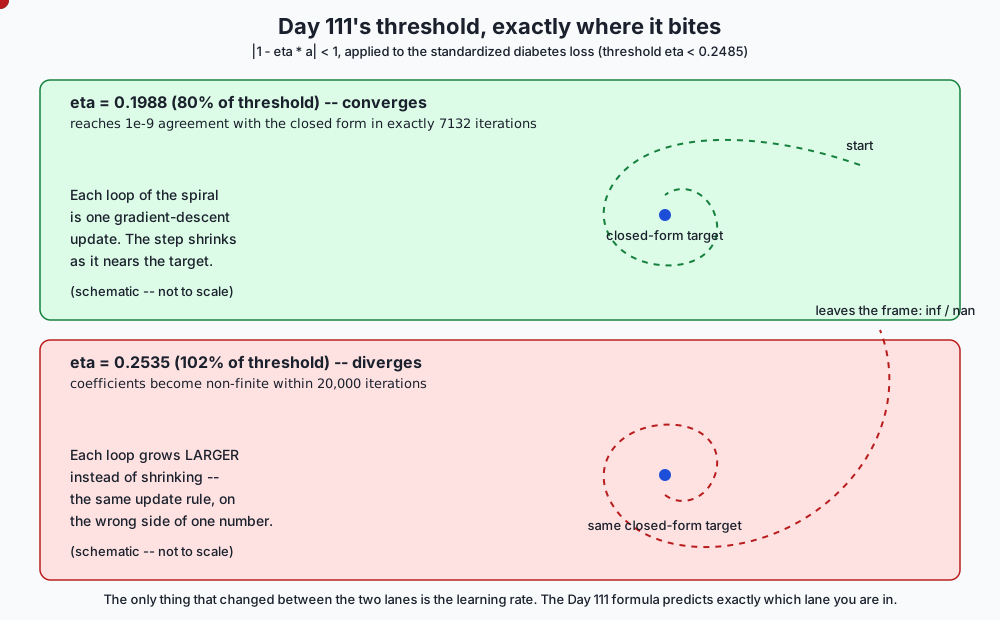
  stability threshold (Day 111, |1 - eta*a| < 1) : 0.2485
  Hessian eigenvalue ratio (max/min)              : 470.08
At a learning rate of 0.2 — about 80 percent of that threshold — gradient descent starting from zero needs:
       decimals of agreement   iterations
                    3               3263
                    6               5277
                    9               7291
Notice the shape of that growth: each additional three decimal places of agreement costs a comparable, not exponentially larger, number of further iterations — roughly two thousand more each time, not a doubling. Gradient descent on a well-conditioned quadratic converges linearly, meaning the error shrinks by a roughly constant factor each iteration, which is exactly why it takes thousands of iterations rather than dozens to reach nine decimal places, but also exactly why it does not take millions.
Then the threshold prediction, tested directly:
  at 80 percent of threshold  (eta=0.1988): converges in 7132 iterations
  at 102 percent of threshold (eta=0.2535): diverges, coefficients non-finite
Two percent over the line, and the same update rule that was steadily homing in on the answer instead grows without bound. Day 111’s formula is not a rough guideline here — it predicts the exact boundary, because it comes directly from the eigenvalues of the actual loss surface being optimized.
Feature scaling: the same condition number, arriving from a different direction
Day 111’s condition number does not only decide the stability boundary — it decides how fast the slowest direction converges once you are safely inside it. And the raw diabetes dataset is, in the terms this course has been using since Week 21, badly scaled on purpose: age in years next to sex coded as 1 or 2 next to serum measurements in the hundreds. Measured directly:
  Hessian eigenvalue ratio, standardized : 470.08
  Hessian eigenvalue ratio, raw features : 76278.96
Over a hundred times worse conditioned, purely from leaving the features in their natural, wildly different units. The consequence, measured rather than assumed: at 95 percent of the RAW data’s own stability threshold — a learning rate chosen specifically to be as aggressive as possible while staying formally stable — gradient descent runs for 200,000 iterations and still has not reached even one decimal place of agreement with the closed form:
  stability threshold, raw features : 4.8746e-04
  after 200,000 iterations, remaining max |coef - closed form| : 0.4692
A learning rate that is stable in principle can still be catastrophically slow in practice, because “stable” only guarantees the largest eigenvalue does not blow up; it says nothing about how many iterations the smallest eigenvalue’s direction needs. This is precisely why standardizing features before running gradient descent is standard practice across the field rather than a stylistic preference: it does not change what the closed form’s answer is, but it can be the difference between thousands of iterations and a number of iterations that never finishes.
What the closed form costs instead
The closed form pays for its speed and its lack of a learning rate with a
different kind of cost: forming X'X is O(n * p^2) and solving it is
O(p^3), where p includes the intercept column. On the diabetes shape,
counted directly rather than timed:
  normal-equation operations (n*p^2 + p^3, n=442, p=11) : 54,813
  gradient-descent operations (2*n*p per iteration, 7291 iterations, n=442, p=10) : 64,452,440
  ratio                                                  : 1175.86x
For this problem’s shape and this convergence target, the closed form
wins by a factor of over a thousand. That comparison flips as p grows:
the p^3 term in the closed form eventually dominates the n * p^2 term,
and at large enough p — hundreds of thousands or millions of parameters
— forming and inverting the matrix at all becomes infeasible regardless of
how fast a single operation is, which is exactly the regime where gradient
descent, and its many refinements, become not merely competitive but
necessary. No wall-clock timing appears anywhere in this comparison, on
purpose: an operation count evaluated by formula is exactly reproducible
on any machine, while a timing is a fact about one run on one machine at
one moment. Section 5 of the lab’s harness asserts the operation counts
directly; it never calls a clock.
fit_intercept, two ways
One implementation detail, resolved by direct comparison rather than
convention: an intercept can be added to the model either by appending a
column of ones to the design matrix and solving the larger system, or by
centring both X and y — subtracting each column’s mean — fitting the
centred, intercept-free problem, and recovering the intercept afterward as
y.mean() - X.mean(axis=0) @ coef. Measured on the diabetes data:
  max |coef_column - coef_centred|         : 1.9554e-11
  |intercept_column - intercept_centred|   : 2.8422e-14
Algebraically the two are exactly the same computation; the measured gap
is pure floating-point rounding, ten to fourteen decimal places down.
OLSRegressor, built for this lab, uses centring, partly because it keeps
the design matrix one column narrower and partly because the two were
worth confirming rather than assuming.
An everyday analogy
Think of the three fitting methods as three different ways to weigh yourself.
The normal equations are a bathroom scale that has you stand on it, then stand on it again holding a second identical scale, and reports the combined reading divided in some particular way. Mathematically that is a correct way to weigh two people. Numerically it is a fragile procedure — if the second scale is even slightly miscalibrated, or if the two people are close to the same weight, the “divided reading” can swing wildly, even though the total is still accurate.
lstsq is a properly calibrated single scale, used directly on each
person. Same physical answer, arrived at by a route that does not amplify
small errors the way stacking two readings does.
sklearn’s default solver is that same properly calibrated scale, plus an extra rule: if the scale genuinely cannot tell two people’s weights apart — because they are, for its purposes, identical — report the split evenly rather than making something up. Not because it secretly knows more about the two people, but because “evenly split” is the most defensible answer among all the ones consistent with what it measured.
Gradient descent is a completely different approach to the same weighing problem: instead of one careful measurement, take a rough initial guess and refine it step by step, nudging your estimate toward whatever the scale’s needle suggests, over and over. Take steps too large — checking the needle so aggressively that you overcorrect each time — and your guess swings further from the truth with every step instead of closer, which is exactly Day 111’s divergence, and exactly what happened at a learning rate two percent over this lesson’s measured threshold. Take appropriately sized steps and you converge, more slowly than reading the scale directly, but reliably.
The analogy earns its keep on the near-duplicate case specifically: weighing two identical twins with a wobbly stacked-scale procedure is exactly the situation where a small measurement error gets amplified into an absurd individual answer, even though the combined weight — the thing you can actually verify — stays correct the whole time.
Examples in practice
Reading NumPy and scikit-learn’s own documentation on this exact question
NumPy’s documentation for numpy.linalg.lstsq describes it as computing
“the least-squares solution to a linear matrix equation,” explicitly via a
singular-value-based method, and separately documents numpy.linalg.solve
for the case where you already have a well-posed square system — which is
precisely the distinction this lesson measures. scikit-learn’s own
developer documentation on LinearRegression states that it uses a solver
appropriate to the least-squares problem and, notably, does not
recommend forming X'X directly for anything but the smallest,
best-conditioned problems — a design choice this lesson’s measurements
justify rather than merely quote.
A design decision this lesson makes concrete
An engineer building a linear model with two features known in advance to
be highly correlated — say, a person’s height in centimetres and their
height in inches, accidentally included twice through a data-pipeline bug
— has, before running any code, already learned the two facts this lesson
measures: the individual coefficients on those two features will not be
reliable no matter which solver is used, and a from-scratch or manually
implemented solver is considerably more likely to return an alarming,
unstable answer than a well-tested library default. The correct response
is not a better solver; it is removing the duplicate column, which is a
data problem, not a numerical one. OLSRegressor’s check_estimator
results, discussed below, illustrate a related but distinct point: a
solver being numerically correct says nothing about whether it validates
its inputs sensibly.
Building OLSRegressor, and citing Day 146 rather than re-deriving it
Day 146 already measured the specific failure a hand-built estimator hits
inside scikit-learn’s own machinery: fit(), predict() and score()
work perfectly well called directly on an object with no scikit-learn
inheritance at all, but Pipeline.predict() and cross_val_score both
raise AttributeError on __sklearn_tags__, a method only BaseEstimator
supplies. OLSRegressor, built for this lesson’s lab, inherits
BaseEstimator and RegressorMixin from the start, for exactly that
measured reason — the API contract itself is not re-taught here.
from sklearn.base import BaseEstimator, RegressorMixin
from sklearn.utils.validation import check_array, check_is_fitted, check_X_y

class OLSRegressor(RegressorMixin, BaseEstimator):
    def __init__(self, method="lstsq", fit_intercept=True, lr=0.1, n_iter=1000):
        self.method = method
        self.fit_intercept = fit_intercept
        self.lr = lr
        self.n_iter = n_iter

    def fit(self, X, y):
        X, y = check_X_y(X, y)
        # ... centre X and y if fit_intercept, then dispatch on self.method
        # to one of the three routes measured in this lesson
        return self

    def predict(self, X):
        check_is_fitted(self, "coef_")
        X = check_array(X)
        return X @ self.coef_ + self.intercept_
Running the real compliance suite, and reporting the real result
sklearn.utils.estimator_checks.check_estimator runs a large battery of
tests against any estimator, checking everything from get_params
round-tripping correctly to behaving sensibly on edge-case inputs like
empty arrays or unusual dtypes. Run against OLSRegressor:
  check_estimator: 48 passed, 2 failed, 2 skipped, 52 total
    FAILED : check_n_features_in_after_fitting
    FAILED : check_dtype_object
    SKIPPED: check_array_api_input (SCIPY_ARRAY_API not set)
    SKIPPED: check_regressor_data_not_an_array (pandas not installed)
Both real failures, named rather than hidden, are about input validation
OLSRegressor does not perform: predict() does not confirm a new X
has the same number of columns the model was fitted on, and fit() does
not reject a malformed y dtype with a clear message. Neither failure is
about the fitting mathematics — OLSRegressor’s coefficients agree with
LinearRegression’s to within 1e-8 or better across all three fitting
methods on this same data. The two skips are environment conditions, not
code defects: one requires an array-API flag this environment does not
set, and the other requires pandas, which is not installed here. Forty-
eight of fifty-two checks passing from a fifteen-line dispatch function and
two inherited base classes is the concrete measurement behind Day 146’s
claim that the API contract is small and deliberately narrow.
Implications: security, privacy, performance, scalability, and cost
A numerically unstable coefficient is a governance risk before it is anything else. If a fitted coefficient feeds a downstream decision — which factor to report as most important, which one a regulator is told the model relies on — a solver that is merely mathematically correct but numerically fragile can hand you a number two hundred thousand times too large, with the opposite sign on its near-duplicate neighbour, and nothing about the fit itself will flag this as wrong. The training loss looks fine. The predictions look fine. Only the coefficients are lying, and only to someone who reads them.
Performance and scalability are where the three methods genuinely
diverge, not merely in decimal places. The closed form’s O(p^3) solve
step is fine at p = 11 and prohibitive at p = 100,000; the same matrix
that costs 54,813 operations here would cost roughly a trillion at that
scale, dominated entirely by the cubic term. Gradient descent’s cost grows
only linearly in p per iteration, which is precisely why every model
with more than a few thousand parameters — essentially all of modern deep
learning — is trained with some variant of gradient descent and never
with a closed-form solve, regardless of how numerically pristine the
closed form would be.
Cost, in the everyday sense, follows the same shape. A closed-form solve on a laptop-scale problem is free in every sense that matters: no tuning, no iteration count to choose, done in one call. Gradient descent’s “cost” is not measured in dollars here but in engineering time — choosing a learning rate, checking convergence, standardizing features first — all of which this lesson’s measurements show are not optional details but the difference between seven thousand iterations and a run that does not converge in two hundred thousand.
Security and privacy connect through the same mechanism Day 150 already raised. A model whose individual coefficients are numerically unstable under near-duplicate or highly correlated features is also a model whose coefficients can be manipulated by an adversary who controls a small amount of the input data — adding a near-duplicate column, deliberately or not, is a lever on the reported coefficients even when it changes predictions almost not at all. The fix — prefer a numerically stable solver, and treat multicollinearity as a data problem to be found and removed — is the same fix that improves both robustness and honest interpretation.
Alternatives: free, open source, and commercial
scikit-learn’s LinearRegression — used here as the referee throughout
When to choose it: for essentially all in-memory ordinary least squares work. Free, BSD-3-Clause licensed, no paid tier. Every measurement in this lesson treats it as the trustworthy reference every from-scratch method is compared against.
How to use it:
from sklearn.linear_model import LinearRegression

model = LinearRegression().fit(X, y)
model.coef_, model.intercept_
Watch for: its default solver choice is deliberately not documented as “the normal equations” anywhere in its public API precisely because the implementation is an internal numerical-stability decision the library reserves the right to improve; relying on its exact solver algorithm rather than its documented behavior is relying on an implementation detail.
NumPy’s numpy.linalg.lstsq and numpy.linalg.solve — used here directly
When to choose them: when you want the least-squares machinery without a scikit-learn dependency, or when building a from-scratch implementation like this lesson’s, where seeing the actual linear-algebra call matters more than convenience. Free, BSD licensed.
How to use them: lstsq for the least-squares problem in general,
solve for a square, well-posed system you already trust to be
invertible:
import numpy as np
coef, *_ = np.linalg.lstsq(X, y, rcond=None)      # least-squares, general case
coef = np.linalg.solve(X.T @ X, X.T @ y)          # normal equations, square system
Watch for: np.linalg.solve on a genuinely singular X'X can raise
LinAlgError, but on a merely ill-conditioned one — including some
near-duplicate cases, verified directly on this machine — it can silently
return a number instead, because floating-point rounding during the matrix
multiplication that forms X'X typically leaves it just shy of exactly
singular. lstsq degrades far more gracefully in this situation, since it
never forms or inverts X'X at all.
statsmodels — described from documentation, not measured here
When to choose it: when the statistical inference around a regression
— standard errors, confidence intervals, hypothesis tests on individual
coefficients — matters as much as the point estimate itself. statsmodels’
OLS class reports these directly. Free, BSD licensed.
Honest note: not installed in the authoring environment this lesson’s lab was built in, and not measured here. Its numerical approach to the underlying least-squares solve is described in its own documentation as similarly careful about conditioning; this lesson does not reproduce output for it and says so plainly.
QR decomposition — described, and the lab’s first extension exercise
When to choose it: a third numerically stable route to the same least-squares answer, distinct from the SVD-based approach sklearn defaults to, that some libraries and textbooks prefer for its lower computational cost relative to a full SVD.
Honest note: not implemented in this lesson’s lab. It is the first
extension exercise, described from numpy.linalg.qr’s documentation
rather than measured here.
Commercial statistical and ML platforms — not used here
Free versus paid: commercial platforms that wrap regression fitting inside a larger analytics or MLOps product typically use the same underlying numerical-linear-algebra libraries (LAPACK and its descendants) under the hood, so the numerical-stability story measured in this lesson applies regardless of which product sits on top. No price is quoted here, because these change by month and an unchecked figure is worse than none; most offer a free tier for individuals and charge for team or enterprise use.
Comparison with related concepts
| Method | What it computes | How it relates |
|---|---|---|
| Normal equations | solve(X'X, X'y) | The textbook formula; squares the condition number, measured here at 1.2153e-10 from sklearn on well-conditioned data and catastrophically far off on the near-duplicate case |
lstsq | Direct SVD/QR-based factorization of X | Never forms X'X; measured about 101x closer to sklearn than the normal equations on the same data |
sklearn LinearRegression | SVD-based minimum-norm solve | The referee this lesson measures everything against; stays sane on the near-duplicate case where the other two explode |
| Gradient descent | Iterative coef -= eta * grad | Needs no matrix inversion, scales to any p; governed by Day 111’s stability threshold, measured here at 0.2485 for this data |
| Ridge regression (Day 151) | Adds alpha * I before solving | A DIFFERENT fix for the same underlying problem — biases the solution deliberately, rather than merely computing the unbiased one more carefully |
| Multicollinearity (Day 150) | The statistical description of correlated predictors | The condition-number squaring this lesson measures is the numerical mechanism behind Day 150’s coefficient instability |
| Condition number | Ratio of largest to smallest singular value | The single number that predicts, before you fit anything, how much precision a given solve route will cost you |
Two rows deserve a closing note.
Ridge regression and a numerically careful solver are not the same
fix, and they are not substitutes for each other. A small ridge penalty,
(X'X + alpha*I)^-1 X'y, genuinely improves the conditioning of the
matrix being inverted — adding alpha*I moves every singular value up by
at least alpha, which directly caps how small the smallest one can be —
but it does this by deliberately introducing bias into the answer, trading
some accuracy for stability. Choosing lstsq over the normal equations
introduces no bias at all; it computes the exact same unbiased answer more
carefully. The lab’s second extension exercise measures how small a ridge
penalty needs to be before it stops the near-duplicate case from
exploding, which is worth doing precisely because the two fixes work by
genuinely different mechanisms.
The condition number is the row that unifies everything else in this
table. Every other row in it is really a statement about how a method
responds to a large condition number — the normal equations amplify its
effect, lstsq and sklearn’s minimum-norm solve dampen it, gradient
descent’s convergence speed is governed by it directly, and ridge
regression improves it by construction. Learning to read a condition
number before fitting anything is the single most transferable skill in
this lesson.
When to use it — and when not to
Use scikit-learn’s LinearRegression, or an equivalent well-tested
library call, for essentially all practical ordinary least squares work.
This lesson exists to show you what it is doing for you, not to talk you
out of using it. The measurements here are an argument FOR trusting a
well-tested numerical library, made by showing precisely what happens
without one.
Implement the normal equations directly only for teaching, for very small and well-conditioned problems, or when you specifically need the derivation on the page. Day 149 used it exactly this way. As a production fitting routine, it is the weakest of the three methods measured here, and the weakness is invisible until a correlated column appears.
Reach for lstsq or an equivalent SVD/QR-based solve when you need
direct control over the linear algebra — inside a from-scratch
implementation, a custom loss combining OLS with something else, or a
research context where seeing every step matters. It is measured here to
be dramatically more trustworthy than the normal equations at essentially
no added conceptual cost.
Reach for gradient descent when the closed form does not fit — too
many parameters for X'X to be invertible in reasonable time or memory,
or a loss that is not quadratic at all, where no closed form exists in the
first place. On a problem this lesson’s size, gradient descent is strictly
the more expensive and more finicky choice, measured directly at over a
thousand times the operation count; its value shows up only once the
closed form stops being an option.
Always standardize features before running gradient descent on a regression problem, unless you have measured, as this lesson did, that your particular data’s raw-scale condition number is already small. The closed form does not need this — it is scale-invariant — but gradient descent’s convergence speed depends on it directly, and the cost of skipping it is measured here at over a hundred thousand iterations of difference.
When you do not need any of this: fitting a single well-conditioned
regression once, with no near-duplicate or highly correlated predictors,
using a maintained library. That is the overwhelming majority of real
regression work, and for it, LinearRegression().fit() is simply the
right answer, chosen for reasons this lesson has now made concrete rather
than assumed.
The AI thread
Everything measured in this lesson scales up, mostly for the worse, at the size of models trained today.
The condition-number story does not go away at scale — it gets harder to see. A neural network’s loss surface has its own local curvature, and badly conditioned directions in that curvature slow training in exactly the qualitative way this lesson measured for a ten-parameter linear regression — except with millions or billions of parameters, nobody computes the full Hessian’s eigenvalues directly, because doing so is itself computationally infeasible at that scale. Practitioners instead watch for the symptom — training that crawls in some directions and diverges in others — without ever seeing the underlying number this lesson computed directly.
Feature and activation scaling is this lesson’s standardization step, running throughout every layer of a large model. Batch normalization, layer normalization and careful weight initialization all exist, in part, to keep the effective condition number of what each layer is optimizing in a range where gradient-based training converges in a reasonable number of steps rather than never. The mechanism this lesson measured on ten diabetes features — raw scale costing over a hundred times the conditioning of standardized scale — is a miniature, fully inspectable version of a problem that shapes the architecture of every large model trained today.
And the from-scratch estimator’s check_estimator result is a small,
concrete instance of a much larger question in AI tooling: what does
“compatible” actually verify? A model or a component can be
mathematically correct at its core task — OLSRegressor’s coefficients
matched sklearn’s to ten decimal places — while still failing basic input
validation that a production system depends on. As more of the AI
pipeline gets assembled from components written by different teams or
different tools, the gap between “does the core computation correctly”
and “handles the inputs a real system will actually throw at it” is
exactly the gap this lesson’s check_estimator run made visible, by name,
rather than by vague reassurance.
Knowledge check
- On well-conditioned diabetes data, the normal equations agree with
sklearn to
1.2153e-10andlstsqagrees to1.1990e-12. Explain where that gap comes from, using the relationship betweencond(X)andcond(X'X). - The near-duplicate-column case sends the normal-equation and
lstsqcoefficients to roughly plus and minus 200,000, while sklearn reports 2.5 and 2.5. State precisely what sklearn’s answer is optimizing for, and why that is not the same as saying it “knows” the true coefficients. - On the same near-duplicate case,
cond(X'X) / cond(X)^2measures at 0.9527 rather than 1.0. Is the underlying theorem false at this condition number, or is something else going on? Explain. - Day 111’s stability condition is
|1 - eta * a| < 1for every Hessian eigenvaluea. At a learning rate 80 percent of the computed threshold, gradient descent converges in 7132 iterations; at 102 percent, it diverges. What single number, computed before running anything, predicts this boundary? - The Hessian eigenvalue ratio is 470.08 on standardized diabetes features and 76,278.96 on raw ones. Both are being fit with a learning rate near their OWN stability threshold. Why does the raw case still converge far more slowly, if it is not diverging?
- The closed form costs 54,813 operations on the diabetes shape; gradient
descent costs 64,452,440 for the iterations measured. Explain why this
comparison uses operation counts rather than wall-clock timing, and
what would happen to the SAME comparison as the number of predictors
pgrows very large. OLSRegressorinheritsBaseEstimatorandRegressorMixin. What specific failure, measured on Day 146 rather than today, does that inheritance prevent?check_estimatorreports 48 of 52 checks passing onOLSRegressor, with 2 named failures. Are those two failures evidence against the coefficientsOLSRegressorcomputes? Explain what they are actually about.
Hands-on exercise
Today’s lab, Linear Regression from Scratch, builds ordinary least
squares three ways in NumPy, wraps them in a scikit-learn-compatible
estimator, and measures every claim in this lesson directly against the
diabetes dataset and a deliberately constructed near-duplicate-column
case.
Ten exercises. The first two build the well-conditioned baseline and
confirm the condition-number-squaring relationship. The next two build the
dramatic near-duplicate case and measure its degraded verification of that
same relationship. The following three apply Day 111’s stability formula
to a real Hessian, measure the raw-versus-standardized slowdown, and
confirm the exact divergence boundary. The last three count operations
instead of timing them, run the real check_estimator suite, and confirm
the two fit_intercept implementations agree.
Build the environment, then work through starter/test_regression_claims.py,
replacing one pytest.skip at a time.
Expected output
The harness ends with:
---------------------------------------------------------------
14 checks, 0 failure(s)
and exits 0. pytest examples -q reports 15 passed, and
pytest starter -q reports 5 passed, 10 skipped until you begin.
The measured table includes:
  max |normal equations - sklearn| : 1.2153e-10
  max |lstsq            - sklearn| : 1.1990e-12
  condition number of X'X / cond(X)^2 : 1.0000000000
  normal-equation coefficients (dramatic case) : [196747.976, ...]
  sklearn coefficients (dramatic case)         : [2.501, 2.0, 2.997, 2.501]
  iterations for 9-decimal agreement, standardized : 7291
  check_estimator: 48 passed, 2 failed, 2 skipped
Validate your work
bash tests/run_tests.sh; echo "exit=$?"reports14 checks, 0 failure(s)andexit=0. Capture the harness’s own exit status..venv/bin/pytest examples -qreports15 passed..venv/bin/python3 examples/report_measurements.py | diff - expected-output/measured-values.txtproduces no output.- When you have finished every exercise,
pytest starter -qreports15 passed. - Break one assertion on purpose, confirm the harness fails, restore it.
Troubleshooting
The 200,000-iteration raw-feature run takes a while. No timing is asserted, so a slow machine changes nothing about whether it passes.
Your exploded coefficients in exercise 2 have different exact digits.
Expected. The magnitude of the explosion is sensitive to the 1e-7 noise
scale, the seed, and even platform floating-point rounding; only the
DIRECTION — both closed forms exceed 1e5 in magnitude, sklearn does not
— is asserted.
cond(X'X) / cond(X)^2 is not exactly 1.0 in exercise 2b. Correct,
and asserted as an inequality rather than an equality, for the reason
worked through in “How it works” above.
import file mismatch. You ran pytest examples starter together.
Run them separately.
Common mistakes
Treating the exploded coefficients as “the normal equations are buggy.” They are not. Both closed-form routes solve the least-squares problem correctly; the explosion is a numerical-stability property of the data’s conditioning, not an implementation error.
Concluding gradient descent is simply worse than the closed form. On
this problem’s size, yes — by a factor of over a thousand in operations.
That conclusion inverts entirely once p grows past what a p^3 solve
can handle, which the lesson states explicitly rather than leaving
implicit.
Quoting cond(X'X) / cond(X)^2 = 1.0 as universally exact in
measurement, not just in theory. The dramatic case measured 0.9527. The
theorem is exact; the floating-point verification of it is not, once
conditioning is extreme enough.
Reading check_estimator’s two failures as evidence the fitting
mathematics is wrong. Both are about input validation, not about the
coefficients themselves, which agree with sklearn to 1e-8 or tighter.
Practice assignment
Take a regression you have already fitted, or fit a small one now, and audit its numerical conditioning.
- Compute
cond(X)for your design matrix, with an intercept column included. If it exceeds a few hundred, treat any individual coefficient’s exact value with real skepticism. - Check for near-duplicate or highly correlated columns, the way Day 150’s variance inflation factor does, or more directly by inspecting the correlation matrix. If two columns correlate above roughly 0.95, expect coefficient instability regardless of which solver you use.
- Refit with
lstsqand with the normal equations, if you have not already confirmed your library uses something in thelstsqfamily by default, and compare the two. A large gap is itself a diagnostic. - If you have ever implemented gradient descent for this problem, compute the Hessian’s eigenvalue ratio and check whether your chosen learning rate sits comfortably below the Day 111 stability threshold, or whether you have simply been lucky.
- State, in one sentence, what “correct” means for your fitted coefficients — predictions that match the data, individual coefficient values that are stable under resampling, or both. This lesson’s central finding is that a solver can deliver the first without the second.
The deliverable is the audit, not a better model.
Extension challenge
Pick one and measure it.
- Nested collinearity. Add a fifth column near-duplicating a different column, so two independent near-collinear pairs exist at once. Measure whether the normal equations’ explosion compounds or stays roughly the same size.
- Ridge as a numerical fix. Refit the dramatic case with
(X'X + alpha*I)^-1 X'yfor a smallalpha, using the normal equations directly. Find how smallalphacan be before the coefficients stop exploding, and report it. - A fourth method: QR decomposition. Implement OLS via
numpy.linalg.qrand measure where it lands relative to the normal equations andlstsqon both the well-conditioned and the dramatic case. - The break-even
p.normal_equation_op_countgrows asn*p^2 + p^3. At a fixedn, find thepwhere thep^3term first exceeds then*p^2term, and explain what that implies for very wide datasets. - Fix one
check_estimatorfailure. Add the missing input validation for eithercheck_n_features_in_after_fittingorcheck_dtype_objectusingsklearn.utils.validationhelpers, and report the new pass count. - A learning-rate schedule. Implement a decaying learning rate and measure whether it lets gradient descent start above the fixed-rate stability threshold without diverging, converging to the same precision in fewer total iterations.
Quiz
Q1. On the diabetes dataset, the normal equations agree with sklearn's LinearRegression to within 1.2153e-10, and lstsq agrees to within 1.1990e-12 -- about a hundred times closer. Both solve the exact same least-squares problem correctly. Where does the gap between them come from?
- The normal equations have a bug: forming X'X loses information a direct solve of X does not
- lstsq uses a different, more accurate loss function than the normal equations
- The normal equations square the condition number of X by forming X'X, so a solve that was already carrying some floating-point error now carries roughly twice as many lost digits
- The gap is measurement noise and would vanish on a different run of the same code
Show answer
Answer: C. The normal equations square the condition number of X by forming X'X, so a solve that was already carrying some floating-point error now carries roughly twice as many lost digits
cond(X'X) is exactly the square of cond(X), measured here as 51631.1119 against 227.2248 squared -- confirmed to ten decimal places. Squaring a condition number roughly doubles how many decimal digits of precision a fixed-precision solve loses. lstsq never forms X'X at all; it factors X directly, so it does not inherit the squared conditioning. Both routes are correct algorithms for the same problem -- there is no bug and no different loss function -- and the gap is deterministic given the pinned software versions, not run-to-run noise.
Q2. Three random columns plus a fourth that is almost identical to the first, true coefficients [1, 2, 3, 4]. The normal equations and lstsq both report coefficients near plus and minus two hundred thousand for the duplicated pair. sklearn's LinearRegression reports 2.5 and 2.5 for the same pair. What is sklearn doing differently?
- sklearn detects the near-duplicate column and silently drops one of them before fitting
- sklearn uses an SVD-based solve that returns the minimum-norm solution among the infinitely many that fit the data almost equally well, splitting the shared weight evenly
- sklearn applies a small amount of regularization by default, which the from-scratch methods do not
- sklearn's LinearRegression is simply wrong here, and the from-scratch answer of plus and minus two hundred thousand is the correct one
Show answer
Answer: B. sklearn uses an SVD-based solve that returns the minimum-norm solution among the infinitely many that fit the data almost equally well, splitting the shared weight evenly
When two columns are nearly collinear, many different coefficient splits fit the data almost equally well -- the true coefficient of 1 shared between the near-duplicate pair could land almost anywhere between them without materially changing predictions. sklearn's default solver finds the minimum-norm answer among those options, which splits the weight evenly at 2.5 and 2.5. LinearRegression does not drop columns and applies no regularization by default (that is Ridge and Lasso's job, covered on Day 151). The exploded from-scratch coefficients are not "more correct" -- they are a numerically unstable answer to an ill-posed sub-problem.
Q3. At the extreme ill-conditioning of the near-duplicate-column dataset, cond(X'X) / cond(X) squared measures at 0.9527, not the 1.0000000000 confirmed on the well-conditioned diabetes data. What does that measured gap mean?
- The theorem cond(X'X) = cond(X) squared is only approximately true, and becomes less true as conditioning worsens
- A bug exists somewhere in the condition-number calculation for extremely ill-conditioned matrices
- The theorem remains exactly true in exact arithmetic; the measured ratio drifts from 1.0 because computing the smallest singular value of an already near-singular matrix is itself numerically imprecise
- The near-duplicate dataset was constructed incorrectly and should be regenerated with a different seed
Show answer
Answer: C. The theorem remains exactly true in exact arithmetic; the measured ratio drifts from 1.0 because computing the smallest singular value of an already near-singular matrix is itself numerically imprecise
cond(X'X) = cond(X) squared is a theorem about singular values, exactly true regardless of how ill-conditioned X is. But VERIFYING it numerically requires computing X's smallest singular value, and when that value is already vanishingly small relative to the largest one -- exactly the situation an extremely ill-conditioned matrix creates -- the computation of that smallest value is itself imprecise. The measurement, not the theorem, degrades. This is the honest finding the lesson reports rather than smoothing over: even a clean mathematical identity can become hard to verify numerically once conditioning is extreme enough.
Q4. Day 111 established that gradient descent on a quadratic loss is stable exactly when |1 - eta * a| < 1 for every eigenvalue a of the loss's Hessian. On standardized diabetes features, that threshold evaluates to eta < 0.2485. What happens at eta = 0.2535, about two percent above the threshold?
- Gradient descent converges slightly more slowly than at eta = 0.2, since it is still fairly close to the threshold
- Gradient descent converges to a slightly different, incorrect answer, since the learning rate is now too large to be accurate
- Nothing changes, since the Day 111 formula is only a rough guideline rather than an exact predictor
- Gradient descent diverges: the coefficients grow without bound and stop being finite numbers within a few thousand iterations
Show answer
Answer: D. Gradient descent diverges: the coefficients grow without bound and stop being finite numbers within a few thousand iterations
Measured directly: at 80 percent of the threshold, gradient descent converges to 1e-9 agreement with the closed form in exactly 7132 iterations. At 102 percent of the threshold, it diverges -- the coefficients become non-finite within 20,000 iterations. The formula is not a rough guideline here; it predicts the exact boundary between the two regimes, because it comes directly from the eigenvalues of the actual loss surface being optimized, not from a heuristic.
Q5. The same gradient-descent setup, run on the RAW (unscaled) diabetes features instead of the standardized ones, has a Hessian eigenvalue ratio of 76278.96 against 470.08 standardized -- over a hundred times worse. At 95 percent of its OWN stability threshold, after 200,000 iterations it still has not reached even one decimal place of agreement with the closed form. Why doesn't a learning rate chosen specifically for the raw features' own threshold fix this?
- The threshold calculation is wrong for unscaled data and needs a correction factor
- The stability threshold only prevents divergence in the direction of the LARGEST eigenvalue; convergence speed in the direction of the SMALLEST eigenvalue is governed by a different, much slower rate
- 200,000 iterations is simply not enough for any dataset; a million would have converged
- Raw features cannot be fit by gradient descent at all, regardless of learning rate
Show answer
Answer: B. The stability threshold only prevents divergence in the direction of the LARGEST eigenvalue; convergence speed in the direction of the SMALLEST eigenvalue is governed by a different, much slower rate
The largest eigenvalue sets the divergence boundary -- exceed it and the loss blows up. But the SLOWEST direction to converge is governed by the SMALLEST eigenvalue, and the condition number (their ratio) determines how many iterations that slow direction needs. A learning rate near the largest-eigenvalue threshold is stable everywhere, but progress along the smallest-eigenvalue direction crawls when that ratio is 76278.96 rather than 470.08. This is Day 111's condition number arriving exactly where it bites, and it is why standardizing features before gradient descent is standard practice rather than a nicety.
Q6. The closed-form solve on the diabetes shape costs 54,813 multiply-add operations (forming X'X plus solving it). Gradient descent, for the 7291 iterations needed to reach 9-decimal agreement, costs 64,452,440 -- about 1176 times more. Why does the lesson count operations rather than timing the two approaches?
- Timing figures depend on the specific machine, CPU load, and hardware they were measured on, so they are excluded from the byte-compared measurement report and would be flaky evidence for anyone reading this on a different machine
- Timing is simply more difficult to implement correctly than counting operations
- Operation counts are always a more accurate measure of real-world speed than wall-clock time
- The two approaches actually run in identical wall-clock time on any modern machine, so timing would show nothing
Show answer
Answer: A. Timing figures depend on the specific machine, CPU load, and hardware they were measured on, so they are excluded from the byte-compared measurement report and would be flaky evidence for anyone reading this on a different machine
A number derived from a formula -- n*p^2 + p^3 against 2*n*p*iterations -- is exactly reproducible on any machine, in any year, regardless of CPU speed, thermal throttling, or what else is running. A wall-clock timing is not: it is a fact about one run on one machine at one moment, and asserting on it produces a test that is flaky everywhere else. Operation counts are not claimed to be a perfect proxy for real-world speed (cache behavior, vectorization and parallelism all matter in practice) -- they are claimed to be the honest, reproducible thing to measure and report here.
Q7. OLSRegressor inherits BaseEstimator and RegressorMixin. Day 146 already measured why a from-scratch estimator needs that inheritance. What was that measured reason?
- Without it, fit() and predict() raise a TypeError immediately when first called
- Without it, the estimator cannot be pickled or saved to disk
- Without it, NumPy refuses to accept the estimator's output as a valid array
- Without it, cross_val_score and Pipeline.predict() raise AttributeError on __sklearn_tags__, a method only BaseEstimator supplies, even though fit(), predict() and score() all work perfectly well called directly
Show answer
Answer: D. Without it, cross_val_score and Pipeline.predict() raise AttributeError on __sklearn_tags__, a method only BaseEstimator supplies, even though fit(), predict() and score() all work perfectly well called directly
Day 146's centrepiece measurement: fit(), predict() and score() work fine on a hand-built estimator with no inheritance at all -- called directly, nothing breaks. The failure appears specifically inside scikit-learn's own machinery (Pipeline.predict() and cross_val_score), which checks for a method named __sklearn_tags__ that only BaseEstimator supplies. This lesson assumes that measurement rather than re-deriving it, and builds OLSRegressor with the inheritance from the start for exactly that reason.
Q8. sklearn.utils.estimator_checks.check_estimator runs 52 checks against OLSRegressor. 48 pass, and 2 fail by name: check_n_features_in_after_fitting and check_dtype_object. What do those two failures indicate about this from-scratch implementation?
- The estimator does not perform certain input-validation steps that scikit-learn's own estimators perform: checking a new prediction's feature count matches training, and rejecting malformed dtypes with a clear error rather than letting an ambiguous failure occur later
- The core fitting mathematics -- the coefficients OLSRegressor computes -- is wrong in some cases
- The estimator is fundamentally incompatible with scikit-learn and cannot be used in a Pipeline at all
- These two failures are false positives caused by a bug in check_estimator itself
Show answer
Answer: A. The estimator does not perform certain input-validation steps that scikit-learn's own estimators perform: checking a new prediction's feature count matches training, and rejecting malformed dtypes with a clear error rather than letting an ambiguous failure occur later
Both failures are about input validation, not about the fitting mathematics -- OLSRegressor's coefficients agree with sklearn's LinearRegression to within 1e-8 or better across all three fitting methods. check_n_features_in_after_fitting checks that predict() rejects data with the wrong number of columns; check_dtype_object checks that malformed input produces a clear error rather than an obscure downstream failure. Both are real, honestly reported gaps in this implementation''s robustness -- not evidence against the 48 checks that DO pass, and not a reason to suppress or hide the two that do not.
Glossary
- Normal equations
- The closed-form solution to ordinary least squares, obtained by solving X'X beta = X'y directly. Textbook-simple, and measured here to agree with sklearn's LinearRegression to only 1.2153e-10 on well-conditioned data -- about a hundred times looser than a direct solve of X.
- lstsq
- A least-squares solve that factors the design matrix X directly rather than forming and inverting X'X. Measured here to agree with sklearn to 1.1990e-12, because it never squares X's condition number the way the normal equations do.
- Condition number
- The ratio of a matrix's largest to smallest singular value, measuring how much a small change in the input can be amplified in the output of a linear solve. 227.2248 for the diabetes design matrix here; 2.4363e+07 for the near-duplicate-column dataset that makes the normal equations explode.
- cond(X'X) = cond(X) squared
- The textbook reason the normal equations lose more precision than a direct solve of X. Confirmed to ten decimal places on well-conditioned data (51631.1119 against 227.2248 squared); the verification itself degrades under extreme ill-conditioning, measured here at 0.9527 rather than 1.0 on the near-duplicate-column case.
- Minimum-norm solution
- Among the infinitely many coefficient vectors that fit an under-determined or near-collinear problem almost equally well, the one with the smallest overall magnitude. sklearn's default LinearRegression solver returns this one, splitting a shared true coefficient of 1 into 2.5 and 2.5 on this lesson's near-duplicate-column dataset rather than exploding.
- Multicollinearity
- Two or more predictor columns carrying overlapping information about each other, first introduced structurally on Day 150. This lesson measures its numerical consequence directly: a near-duplicate column sends closed-form coefficients past 196,000 in magnitude while the true coefficients are 1 and 4.
- Gradient-descent stability threshold
- The learning rate above which gradient descent on a quadratic loss diverges, from Day 111's condition |1 - eta * a| < 1 applied to the loss's largest Hessian eigenvalue. Measured at 0.2485 for standardized diabetes features; gradient descent converges in 7132 iterations at 80 percent of it and diverges to non-finite values at 102 percent.
- Hessian eigenvalue ratio
- The condition number of the loss surface gradient descent is optimizing, governing how many iterations the slowest direction needs to converge. 470.08 on standardized diabetes features; 76278.96 on raw, unscaled ones -- over a hundred times worse, which is why gradient descent barely moves on badly scaled data even at a stable learning rate.
- Feature standardization
- Rescaling every column to zero mean and unit standard deviation before fitting. Not required for the closed form, which is invariant to scale, but measured here to shrink the Hessian eigenvalue ratio from 76278.96 to 470.08 and make gradient descent converge in thousands of iterations rather than hundreds of thousands.
- Operation count
- Multiply-add operations computed by formula rather than timed on a clock, so the comparison survives a different machine unchanged. 54,813 for the closed form on the diabetes shape against 64,452,440 for gradient descent to reach 9-decimal agreement -- about 1176 times more.
- BaseEstimator
- The scikit-learn base class supplying get_params, set_params and __sklearn_tags__ by introspecting __init__. Day 146 measured that a from-scratch estimator raises AttributeError inside Pipeline.predict() and cross_val_score without it, even though fit, predict and score work fine called directly; OLSRegressor inherits it for that measured reason.
- RegressorMixin
- A scikit-learn mixin supplying a default score() method (R-squared) for any estimator that implements predict(). Paired with BaseEstimator on OLSRegressor so it behaves as a complete regressor rather than a bare fit/predict object.
- check_estimator
- scikit-learn's own compliance suite for a hand-built estimator. Run against OLSRegressor here: 48 of 52 checks pass; the two failures, named rather than suppressed, are both about input validation this implementation does not perform.
- fit_intercept by centring
- Computing an intercept by subtracting each column's mean before fitting and recovering it afterwards as y.mean() minus X.mean(axis=0) dotted with the coefficients, rather than appending a column of ones to the design matrix. Measured here to agree with the column-append approach to within 1.9554e-11 on coefficients and 2.8422e-14 on the intercept.
- Singular versus ill-conditioned
- A singular matrix cannot be inverted at all; an ill-conditioned one can be inverted but the inversion amplifies floating-point error. The near-duplicate column in this lesson's dramatic case is ill-conditioned, not exactly singular -- which is why the normal equations return a number at all, just a badly wrong one.
- SVD-based solve
- A least-squares solution method built on the singular value decomposition, which sklearn's default LinearRegression uses. Directly exposes a matrix's small singular values, letting it return the minimum-norm answer on near-collinear data rather than the exploded answer the normal equations and a naive lstsq both fall into on the most extreme cases.
- Batch gradient descent
- The update rule coef := coef - eta * gradient, applied to every row of the data on every iteration. Day 111's material, applied here to ordinary least squares' mean-squared-error loss, whose gradient is (2/n) X'(X coef - y).
Sources and further reading
- numpy.linalg.lstsq -- NumPy API reference — NumPy developers (accessed 2026-08-27)
- numpy.linalg.solve -- NumPy API reference — NumPy developers (accessed 2026-08-27)
- numpy.linalg.cond -- NumPy API reference — NumPy developers (accessed 2026-08-27)
- LinearRegression -- scikit-learn API reference — scikit-learn developers (accessed 2026-08-27)
- Developing scikit-learn estimators -- the API contract check_estimator verifies — scikit-learn developers (accessed 2026-08-27)
- check_estimator -- scikit-learn API reference — scikit-learn developers (accessed 2026-08-27)
- load_diabetes -- scikit-learn API reference, including scaled vs raw units — scikit-learn developers (accessed 2026-08-27)
- Condition number — Wikipedia (accessed 2026-08-27)
- Ordinary least squares — Wikipedia (accessed 2026-08-27)
- The Elements of Statistical Learning, chapter 3 on linear methods for regression -- free PDF from the authors — Trevor Hastie, Robert Tibshirani and Jerome Friedman, Springer (accessed 2026-08-27)
Kept in this browser, no account needed. Your progress page turns the whole record into one link you can bookmark or open on another device.