Machine Learning › Regression › Day 154
Day 154: A Complete Regression Project

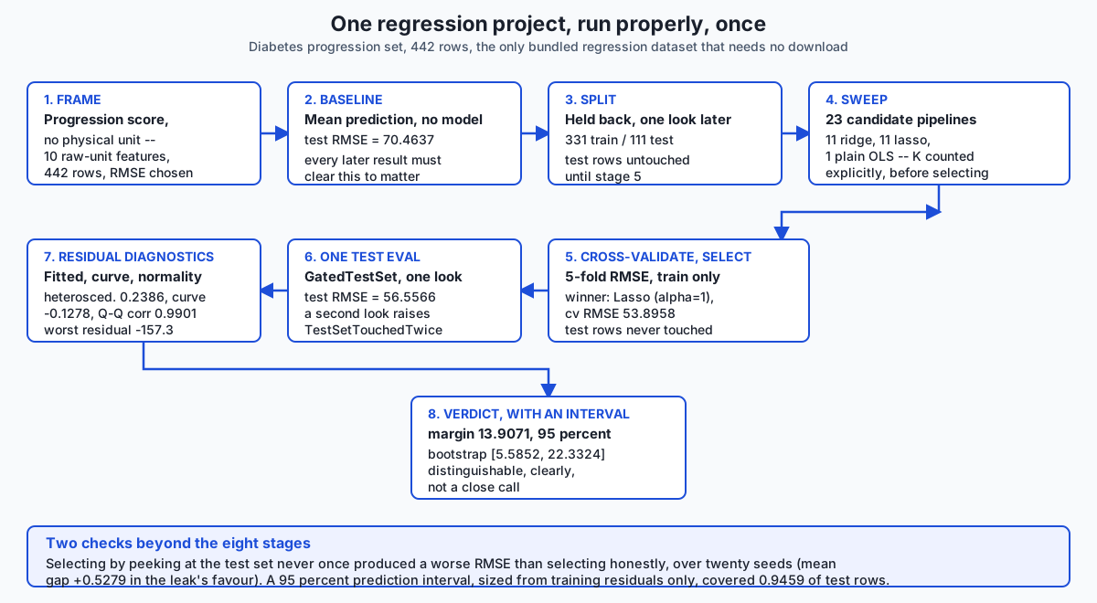
After this lesson you will have run one regression project properly, once, on a real dataset, and watched six days of separate disciplines pay off together instead of in isolation. You will compute a mean-predictor baseline before fitting anything, sweep 23 real candidate pipelines -- ridge, lasso and plain OLS -- and select a winner by cross-validating on training rows only. You will evaluate the test set exactly once through a mechanical gate, and compute a 95 percent bootstrap interval around the winning model's margin over baseline -- 13.9071 RMSE points, comfortably clearing an interval of [5.5852, 22.3324]. You will read residual diagnostics as this day's centrepiece: a mild heteroscedasticity signal, a weak curvature signal, a from-scratch normal-probability check, and the five largest individual mistakes named and inspected. You will measure whether the model is worse for high-value targets than low-value ones on a disease-progression score, and find the answer is nearly flat rather than assuming it either way. You will reconstruct, deliberately, the mistake of selecting a model by scoring every candidate directly against the test set, and watch the resulting gap never once turn negative across 20 seeds. And you will build a prediction interval from held-out residuals and measure its realised coverage -- 0.9459 -- against its 0.95 nominal rate, rather than trusting the nominal number on faith.
Hands-on lab for this lesson
Lab files on GitHub: https://github.com/ai-roadmap-365/ai-roadmap-365.github.io/tree/main/labs/sections/machine-learning/day-154-a-complete-regression-project
- Get the hands-on files. Clone the labs repository once (you can reuse this clone for every lesson). This works on macOS, Linux, and Windows (PowerShell or WSL):
git clone https://github.com/ai-roadmap-365/ai-roadmap-365.github.io.git cd ai-roadmap-365.github.io - Open this lesson's lab. Move into the directory for this specific day. Every lab lives at the same predictable path — section / subsection / week / day:
cd labs/sections/machine-learning/day-154-a-complete-regression-project - Read the lab guide. Open `README.md` in that directory. It lists the exact commands, what each does, the expected output, and how to check your work — read it before running anything.
- Run it and check your work. Follow the README's "How to run" section: run the example first to see the finished result, then complete the numbered exercises in `starter/`, then run the tests. The tests pass (exit 0) only when your work is correct.
bash tests/run_tests.sh # or the test command named in the lab README
You can also open the lab as a local page (works offline, shows the file tree and expected output).
Learning objectives
By the end of this lesson you will be able to:
- Choose a regression dataset by what is genuinely available offline, and state plainly when a target has no physical unit
- Compute a mean-predictor baseline before fitting any model, and use it as a gate every later result must clear
- Build a train/test split sized honestly for a small dataset, and hold the test rows back until exactly one evaluation
- Sweep a real set of candidate pipelines with scikit-learn's Pipeline, and count K explicitly rather than losing track of it
- Select a winning configuration using cross-validation on training rows only, choosing RMSE as the metric before any model is fitted
- Evaluate a test set exactly once with a mechanical gate, reusing the GatedTestSet pattern from Day 144 and Day 147
- Compute a bootstrap interval around a model's margin over baseline, and judge whether an improvement is distinguishable from noise at the test-set size actually available
- Read residual-vs-fitted, curvature and normal-probability diagnostics as the centrepiece of a regression verdict, not an afterthought to a single RMSE
- Measure whether a model's errors are worse for high-value targets than low-value ones, and report the result honestly whichever way it comes out
- Reproduce the mistake of selecting a model by scoring every candidate directly on the test set, and explain why the resulting gap can never be negative
- Build a prediction interval from held-out training residuals, and measure its realised coverage against its nominal rate rather than assuming the two match
- Assemble frame, baseline, split, pipeline, cross-validation, selection, one test evaluation, residual diagnostics, a fairness check and prediction intervals into a single defensible verdict
Prerequisites
- Day 144 -- the three sets, the selection-optimism formula, and the GatedTestSet pattern this lesson reuses
- Day 147 -- the full classification protocol this lesson mirrors for regression, and the leaky-selection mistake this lesson reconstructs a second time
- Day 148 -- the one-predictor linear model, coefficient interpretation in real units, and the four assumptions this lesson's residual diagnostics check
- Day 149 -- the loss as a choice, and why squared error and absolute error can disagree about which model is best
- Day 150 -- multicollinearity, measured on this exact dataset, needed to read why regularisation helps prediction only modestly here even though it stabilises coefficients dramatically
- Day 151 -- ridge and lasso, the two regularised families this lesson's sweep is built from
- Day 152 -- metrics that can be gamed or inverted, needed to trust that RMSE was chosen here as a considered choice rather than a default
- Day 153 -- OLS built from scratch, and comfort with NumPy arrays and reading a pytest failure; a working python3 3.11 or newer on your PATH; the lab builds its own virtual environment and needs no GPU
Why this matters
Here is a number that should stop you before you write a single line of code: 70.4637.
That is the RMSE of the simplest possible regression model on today’s dataset — guess the training mean for every patient, no features, no fitting, nothing. If you build a careful pipeline, sweep two dozen candidates, cross-validate honestly, and report a test RMSE of, say, 68 — a number that sounds like progress — you have built something worse than guessing the mean, dressed up in enough machinery to look like it isn’t. Nobody who skips the baseline finds this out. They just report “68 RMSE” and move on, and the number means nothing at all, because nothing was ever compared against anything.
That is the concrete failure this lesson opens with, and it happens constantly, in student projects and production systems alike: a regression model gets built, a number gets reported, and the number is never checked against the one thing that would tell you whether it is worth anything. Today you build the whole check, once, on 442 rows of real measurements from real patients, predicting a disease-progression score with no name — no mg/dL, no dollars, no physical unit at all — and you find out exactly how much six days of separate lessons buy you when they are spent together instead of in isolation.
Here is the headline result, computed before you read another paragraph
so you can watch the arithmetic earn it rather than take it on faith. A
sweep of 23 candidate pipelines — 11 ridge strengths, 11 lasso strengths,
one plain OLS — cross-validated honestly on training rows, selects
Lasso(alpha=1) at a cross-validated RMSE of 53.8958. Evaluated exactly
once against 111 held-back test rows, it scores 56.5566 RMSE — a margin
of 13.9071 points over the 70.4637 baseline. A bootstrap interval around
that margin, built by resampling the test set two thousand times, comes
out to [5.5852, 22.3324]. The interval does not cross zero. On this
small, real, honestly-evaluated dataset, the model is genuinely,
measurably better than guessing — not by a landslide, but by more than
sampling noise on 111 rows could plausibly explain. That is a verdict,
not a hunch, and every number in it came from code you can re-run.
Days 148 through 153 taught you the pieces one at a time: a one-predictor line and its four assumptions, the loss function as a deliberate choice rather than a default, what correlated predictors do to a coefficient, what ridge and lasso do about it, how RMSE and R² can be gamed or can flatly disagree, and how the normal equations actually compute a line from scratch. None of those lessons told you what happens when you run all of them together, in the order a working project actually needs them, and read the result honestly — including the parts that come out smaller, flatter, or more boring than you might have guessed. Today is that lesson, and its centrepiece — reading the residuals themselves rather than stopping at one RMSE — is something no earlier day in this course has owned.
The idea in plain language
Think about a structural engineer signing off on a bridge design.
An engineer who says “the load calculation checks out” and stops has not finished the job, even if the calculation is correct. A complete sign-off states the baseline case — what happens if you build nothing, or the simplest possible structure — walks through the specific loads actually modelled, states the margin of safety with a number attached, not just a pass/fail, and then does the part that separates a real inspection from a rubber stamp: looks at where the stress concentrates. Not “does the bridge hold,” but “where would it fail first, and by how much load would it take.” An engineer who reports a single safety factor and nothing else has produced a number, not an inspection.
That is what today’s protocol is, applied to a regression model instead of a bridge. Frame is stating exactly what you are predicting, from what, in what population, and — critically for today’s dataset — whether the number you are predicting even has a unit that means something outside the model. Baseline is the load case of building nothing: how wrong would you be if you just guessed the average, every time? Split is deciding which measurements inform your design and which one you hold back to check yourself against, once, at the end. Sweep and cross-validate is trying several structural approaches and scoring each one honestly, on cases you’re allowed to reconsider. Select is committing to the design that scored best, understanding that “scored best” is itself a number with some wobble in it. One test evaluation is the single, final load test — run once, not adjusted and re-run until it passes. Residual diagnostics is the part a bare safety factor skips entirely: not “did it hold,” but “where does it strain, does the strain grow with the load, and what do the worst five failure points actually look like.” A fairness check is asking whether the structure is disproportionately weaker under one kind of load than another. Prediction intervals replace a single point estimate — “this beam holds 40 tons” — with an honest range, and then checks that range against reality rather than trusting the formula that produced it. Verdict is all of that, together, with an interval attached to the headline number rather than a bare percentage.
Six days ago you learned pieces of this inspection in isolation. Today you run the whole inspection, on a real structure — a real dataset — and you find that some of what you’d expect from the textbook holds up exactly, some of it holds up only modestly, and one of it (the fairness check) comes back nearly flat, which is itself a finding worth having, not a disappointment to explain away.
Historical background
The individual pieces of today’s protocol each have their own history, which earlier days in this course already told properly — cross- validation back to Geisser and Stone in 1974, the three-set discipline and selection optimism from Day 144, ridge regression’s origin in Hoerl and Kennard’s 1970 paper on dealing with correlated predictors, lasso’s introduction by Tibshirani in 1996. Today’s history is different in kind: it is the history of the dataset itself, because an end-to-end exercise has to be honest about where its numbers came from.
The diabetes dataset — load_diabetes in scikit-learn — comes from a
2004 paper by Bradley Efron, Trevor Hastie, Iain Johnstone and Robert
Tibshirani, “Least Angle Regression,” published in The Annals of
Statistics. The paper introduced LARS, a computationally efficient
algorithm related to lasso, and used this dataset of 442 diabetes
patients as its running example. Ten baseline variables — age, sex, body
mass index, average blood pressure, and six blood serum measurements —
were recorded for each patient, along with a quantitative measure of
disease progression one year after baseline. That progression measure is
the target this lesson predicts, and it is worth being precise about
what it is: a composite clinical score assembled from several measures
of diabetes progression, with no independent physical meaning outside
the study that defined it. It is not measured in units of anything a
reader would recognise, and this lesson says so rather than inventing a
plausible-sounding unit to make the numbers feel more concrete than they
are.
Because the dataset comes from a statistics methodology paper rather
than a raw clinical dataset, scikit-learn bundles it in two forms. The
package’s own default, scaled=True, returns every feature mean-centred
and scaled by its standard deviation times the square root of the sample
size — a transformation useful for comparing regularisation paths across
features of different natural scales, but one that turns “age” into a
number between roughly -0.11 and 0.11 with no year attached. This lesson
asks for scaled=False instead, which recovers the original measurement
units: age in years, blood pressure and the serum measures in their
original clinical scales. The reason matters and connects directly to
Day 148: a coefficient computed on raw units means something a human can
sanity-check — “one additional year of age is associated with this many
points of progression” — while a coefficient on the scaled version means
something only in the abstract, standardised sense the paper’s authors
needed for their own comparison. load_diabetes needs no network
connection, unlike fetch_california_housing, scikit-learn’s other
bundled regression dataset, which downloads on first use — a fact this
lesson checks directly rather than assuming, because this lab’s safety
rule forbids any network access beyond the one initial package
installation.
The methodological history is the more directly relevant one. The discipline of running a full, documented modelling pipeline — frame, split, cross-validate, one test evaluation, residual analysis, a stated verdict with an interval — rather than reporting whichever number a search process happened to surface, developed in applied statistics specifically because residual analysis has always been understood, since at least the mid-twentieth-century development of regression diagnostics by statisticians like John Tukey and Frank Anscombe, as inseparable from a regression fit. Anscombe’s 1973 quartet — four datasets with nearly identical summary statistics and wildly different underlying structure, visible only once you plot the residuals — is the classical demonstration that a fit statistic alone can systematically mislead. Today’s lesson inherits that discipline directly: the residual diagnostics section is not a bonus feature bolted onto a regression project. Historically, and in this lesson, it is the point.
What it is — and what it is not
A complete regression project is the assembly of prior disciplines
into one protocol, applied to one real dataset, producing one written
verdict with residual diagnostics at its centre. It is not a new
algorithm — every estimator used today (Ridge, Lasso,
LinearRegression) was already available by Day 151, and the
GatedTestSet pattern is unchanged from Day 144.
Here is what today’s protocol precisely is, stage by stage.
Frame states, in one sentence, what is being predicted, from what
features, and whether the target has a unit at all. For this lesson:
disease-progression score (unitless, composite) from 10 clinical
measurements in raw units, in the population represented by the 442 rows
of load_diabetes.
Baseline is the score of the simplest possible non-model: predict the training mean for every row. Here, 70.4637 RMSE, -0.0001 R² — computed before any real model is fitted, so it can act as the gate every later result has to clear.
Split divides the 442 rows into 331 training rows and 111 test rows, with the test rows held back from everything until stage six. 111 rows is small — small enough that every interval this lesson computes is wide — and that is reported honestly rather than smoothed over.
Sweep and cross-validate builds K = 23 candidate pipelines — 11
values of the regularisation strength alpha for ridge, 11 for lasso,
and one plain OLS — and scores every one of them with 5-fold
cross-validation on the 331 training rows, using RMSE as the metric,
chosen deliberately before any candidate is fitted. No candidate ever
sees a test row during this stage.
Select picks the lowest cross-validated RMSE: Lasso(alpha=1), at
53.8958.
One test evaluation fits that winning configuration on the full 331 training rows and scores it, exactly once, against the 111 held-back rows, wrapped in a gate that refuses a second look. The result: 56.5566 RMSE, 0.3557 R², 45.2846 MAE.
Residual diagnostics — this lesson’s centrepiece — reads the actual errors, not just their RMSE summary. A heteroscedasticity signal of 0.2386 (a mild tendency for errors to grow with the prediction), a curvature signal of -0.1278 (weak, no strong missed trend), a normal-probability correlation of 0.9901 (close to a straight Q-Q line), and the five largest individual mistakes, inspected by name.
A fairness check splits the test set at the median true value and compares RMSE on each half: 55.2464 below, 57.8601 above, a ratio of 1.0473 — nearly flat.
Prediction intervals build a range around each prediction from training residuals, and measure the realised coverage on the test set: 0.9459, against a 0.95 nominal rate.
Verdict states a bootstrap interval around the margin over baseline — [5.5852, 22.3324] around a margin of 13.9071 — and, separately, reconstructs the leaky-selection mistake to show what happens when the test set is used to select rather than to confirm: a mean gap of 0.5279 RMSE points in the leak’s favour over 20 seeds, never negative.
Now the things this exercise is not.
It is not a demonstration that regularisation dramatically fixes multicollinearity’s practical impact. Day 150 measured VIFs as high as 59.2 on this exact dataset’s raw features — real, severe multicollinearity. Today’s sweep shows that plain OLS, with no regularisation at all, scores only 0.1968 RMSE points worse than the regularised winner in cross-validation. Multicollinearity destabilises individual coefficients dramatically, as Day 150 showed; it does not necessarily destabilise predictions by anywhere near as much, because correlated predictors can substitute for one another in the fitted equation even as their individual weights swing wildly. Both facts are true at once, and today’s measurement is what tells you which one applies to prediction accuracy versus coefficient interpretation.
It is not evidence that residual diagnostics always come back alarming. The heteroscedasticity and curvature signals measured here are real but modest — not the textbook-perfect flat scatter, but also not a dramatic funnel or a visible curve. A learner who expects residual diagnostics to always either “pass cleanly” or “reveal a crisis” has missed the more common real case: a small, genuine signal that is worth noting and watching, neither ignored nor treated as disqualifying.
And it is not a clinical tool. A 56.5566 RMSE, evaluated once on 111 rows of a dataset originally assembled for a 2004 statistics methodology paper, is a pedagogical result about a modelling protocol applied to a score with no independent physical meaning. Reading it as evidence about how well machine learning predicts real diabetes progression would be exactly the kind of unjustified leap this course has tried to train you out of making.
Why it was created and what problems it solves
Each of today’s stages exists because a specific, nameable failure happens when it is skipped, and every one has already been measured this week — today’s contribution is showing that they compound, in order, in one real regression pipeline.
Skipping frame and baseline produces a number with no reference point — the 68-RMSE trap this lesson opened with. A model that reports “68 RMSE” sounds like it did something until you learn the mean-predictor baseline gets 70.4637 for free: barely better than guessing, dressed up in machinery.
Skipping the split, or splitting after fitting something, is Day 143’s stage-ordering failure, still binding here: a scaler that has seen test rows, or a hyperparameter search that peeked, leaks information into every downstream decision.
Skipping cross-validation in favour of a single validation split reintroduces the holdout-variance problem Day 144 measured directly on a different dataset. Cross-validating the 23-candidate sweep here is what makes the winner’s cross-validated RMSE, 53.8958, a stable enough number to select on rather than a single lucky split’s noise.
Skipping the residual diagnostics is this lesson’s own central warning. A model can post a respectable RMSE while its errors quietly fan out with the prediction size, or cluster in a way a single summary number cannot show. Today’s 0.2386 heteroscedasticity signal is not dramatic enough to disqualify the model, but a reader who never checked would not know that — they would simply not know, which is worse than knowing the answer is “modest but real.”
Skipping the fairness check by target level hides exactly what today’s measurement reveals: whether a model’s errors concentrate on the patients with more severe outcomes. Here the answer is reassuring — a 1.0473 ratio, nearly flat — but the check had to run for that reassurance to mean anything. An unchecked model could just as easily have shown a ratio of 1.5 or 2.0, and nobody would have known without measuring.
Skipping the interval around the margin turns a verdict into a guess dressed as a fact. Day 144 built the machinery for classification accuracy; today extends it to RMSE with a bootstrap, because RMSE has no equally simple closed-form standard error. Applied here: is 13.9071 RMSE points of improvement meaningfully better than zero, given only 111 test rows? The interval says yes, clearly. It could easily have said no, on a smaller improvement or a smaller test set — which is exactly why the bootstrap runs rather than being assumed.
Skipping the prediction interval’s coverage check is a subtler version of the same mistake. A model can report a “95 percent prediction interval” that, in practice, covers 70 percent of real outcomes or 99 percent of them — nobody knows unless the realised coverage is measured against the nominal rate, exactly as today’s 0.9459-versus-0.95 comparison does.
And skipping the discipline that keeps the test set honest — using it to select rather than to confirm — is the mistake exercise 10 reconstructs directly, this time for regression rather than classification. It is, in the applied-ML literature and in real teams, probably the single most common way a reported number ends up inflated: not a dramatic leak, just quietly trying a few configurations against the number you eventually report.
How it works
Choosing the dataset, by what is genuinely available
sklearn.datasets bundles exactly one regression dataset that needs no
download: load_diabetes. Its counterpart,
fetch_california_housing, downloads its data file on first use —
inspect.signature(fetch_california_housing).parameters['download_if_missing'].default
is True, confirmed directly rather than assumed. Because this lab’s
safety rule forbids any network reach beyond the one initial package
install, load_diabetes is not a stylistic preference here; it is the
only option that satisfies the constraint.
scaled=False is the second deliberate choice. scikit-learn’s own
default, scaled=True, returns every feature mean-centred and scaled to
tiny floats — age between roughly -0.11 and 0.11, with no year attached.
scaled=False recovers the original clinical units: age in years (19 to
79 in this dataset), body mass index and blood pressure in their
original scales. Day 148’s point about coefficient interpretation only
means anything if a coefficient is computed in units a reader can
sanity-check, so this lesson asks for the raw version.
The frame, and the baseline
The frame is one sentence: predict a composite disease-progression
score — no physical unit — from 10 real-valued clinical measurements. The
baseline is one function call — DummyRegressor(strategy="mean") — fitted
on the training rows and scored on the held-back test rows:
mean-predictor baseline: RMSE 70.4637, R2 -0.0001Every later number in this lesson is read against 70.4637.
The split
train_test_split(X, y, test_size=0.25, random_state=0) gives 331
training rows and 111 test rows. A 25 percent test set on 442 total rows
is small on purpose — small enough that every interval computed below is
wide, and that width is the honest consequence of the data available,
not a flaw in the method.
The sweep
Twenty-three candidate pipelines, built with scikit-learn’s Pipeline so
StandardScaler is refit inside every cross-validation fold rather than
fitted once on everything — Day 143’s ordering rule, enforced by the
estimator’s own contract:
from sklearn.pipeline import Pipeline
from sklearn.preprocessing import StandardScaler
from sklearn.linear_model import Ridge, Lasso, LinearRegression

alphas = [0.001, 0.003, 0.01, 0.03, 0.1, 0.3, 1, 3, 10, 30, 100]

configs = []
for a in alphas:
    configs.append(("ridge", a, lambda a=a: Pipeline([
        ("scale", StandardScaler()), ("clf", Ridge(alpha=a)),
    ])))
for a in alphas:
    configs.append(("lasso", a, lambda a=a: Pipeline([
        ("scale", StandardScaler()), ("clf", Lasso(alpha=a, max_iter=20000)),
    ])))
configs.append(("ols", 0.0, lambda: Pipeline([
    ("scale", StandardScaler()), ("clf", LinearRegression()),
])))
That is K = 23, counted, not estimated.
Cross-validate, then select — with the metric decided first
RMSE is chosen as the selection metric before any candidate is fitted — Day 152’s whole argument that the metric is a choice, made concretely here, in the target’s own unitless composite-score points rather than some borrowed unit that does not apply:
from sklearn.model_selection import KFold, cross_val_score

splitter = KFold(n_splits=5, shuffle=True, random_state=0)
scored = [
    (family, param, -cross_val_score(make(), x_train, y_train,
        cv=splitter, scoring="neg_root_mean_squared_error").mean())
    for family, param, make in configs
]
scored.sort(key=lambda row: row[2])
winner_family, winner_param, winner_cv_rmse = scored[0]
The winner: Lasso(alpha=1), cross-validated RMSE 53.8958. Plain OLS
scores 54.0926 at the same seed — only 0.1968 points behind, even though
Day 150 measured VIFs as high as 59.2 on these exact features.
Multicollinearity’s dramatic effect was on individual coefficients, not
on this margin.
One test evaluation, gated
class GatedTestSet:
    def evaluate(self, model):
        if self.evaluations >= 1:
            raise TestSetTouchedTwice(...)
        self.evaluations += 1
        pred = model.predict(self._X)
        return rmse, r2, mae   # computed once, from this one prediction
Fitting the winner on the full 331 training rows and calling
gate.evaluate(fitted) once gives:
test RMSE: 56.5566 R2: 0.3557 MAE: 45.2846A second call raises TestSetTouchedTwice.
The margin, with a bootstrap interval
The margin over baseline is 70.4637 - 56.5566 = 13.9071 RMSE points.
Because RMSE has no equally simple closed-form standard error the way a
proportion does, the interval around that margin comes from resampling
the 111 test rows with replacement 2000 times, recomputing both RMSEs on
each resample:
margin = baseline_rmse - model_rmse = 13.9071
95 percent bootstrap interval on the margin: [5.5852, 22.3324]
The interval’s lower bound, 5.5852, is comfortably positive: this model’s improvement is distinguishable from zero at this test-set size. It could easily have come out otherwise, on a smaller improvement or a smaller test set — that is precisely why the bootstrap runs rather than being assumed.
Residual diagnostics: the centrepiece
This is the part of the protocol no earlier day owns, and it is where today’s real attention goes.
Residual mean and spread. The 111 test residuals average -3.6262 with a standard deviation of 56.4402 — centred close to zero, as a reasonably well-fit model’s residuals should be.
Heteroscedasticity — do errors grow with the prediction? Measured as the correlation between the fitted value and the absolute residual:
heteroscedasticity signal, corr(fitted, |residual|): +0.2386A value of exactly zero would mean error size is unrelated to the prediction; ±1 would mean a dramatic, unmissable funnel. 0.2386 is real — not zero — but modest: a mild tendency for larger predictions to carry somewhat larger errors, worth watching rather than alarming.
Curvature — is there a missed non-linear trend? Measured as the correlation between the squared fitted value and the signed residual:
curvature signal, corr(fitted^2, residual): -0.1278Weak. No strong evidence that a linear model is missing an obvious curve in this data.
Normal probability — are the residuals shaped like a bell curve? A from-scratch Q-Q correlation, built without scipy (not one of this lab’s three pinned dependencies) using a rational approximation to the inverse normal CDF:
normal-probability (Q-Q) correlation: 0.99011.0 would be a perfectly straight Q-Q line. 0.9901 is close: these residuals are close to normally distributed, even on real data with only 111 test rows — a genuinely reassuring result for a model whose interval arithmetic (both the margin bootstrap and the prediction interval below) implicitly leans on residuals not being wildly non-normal.
The five largest individual mistakes, named:
row  60: true=   52.0  pred=  209.3  residual=  -157.3
row  65: true=  302.0  pred=  153.9  residual=  +148.1
row  24: true=   68.0  pred=  202.8  residual=  -134.8
row   9: true=   99.0  pred=  230.1  residual=  -131.1
row  64: true=  132.0  pred=  261.3  residual=  -129.3
An RMSE of 56.5566 does not tell you that this model’s worst single mistake is a patient predicted at 209.3 whose true progression score was 52.0 — a residual nearly three times the RMSE itself. Reading the largest individual residuals, not just the summary statistic, is how you find out a model has specific, severe failure modes rather than uniformly moderate error.
Is the model worse for high-value targets? Measured, not assumed.
RMSE on below-median targets: 55.2464
RMSE on above-median targets: 57.8601
ratio (high / low): 1.0473
Only 4.73 percent worse on the more severe half of test cases at this seed. On a disease-progression score, this is a fairness-relevant question, not only a statistical one — is the model systematically less accurate for patients whose condition has progressed further, which is exactly the group where an accurate prediction might matter most? The honest answer here is nearly flat. That is a real finding: the check had to run for the reassurance to mean anything, and a different dataset, or a different seed, could easily have surfaced a larger asymmetry.
The leaky version, run alongside the honest one
Reconstructing Day 147’s central mistake, for regression: selecting a model by fitting every candidate and scoring it directly on the test set, keeping whichever produces the lowest RMSE, instead of selecting on cross-validated training rows and looking at test once.
def leaky_selection_test_rmse(x_train, y_train, x_test, y_test):
    best_rmse = None
    for _family, _param, make in configs:
        pipe = make().fit(x_train, y_train)
        rmse = compute_rmse(y_test, pipe.predict(x_test))
        if best_rmse is None or rmse < best_rmse:
            best_rmse = rmse
    return best_rmse
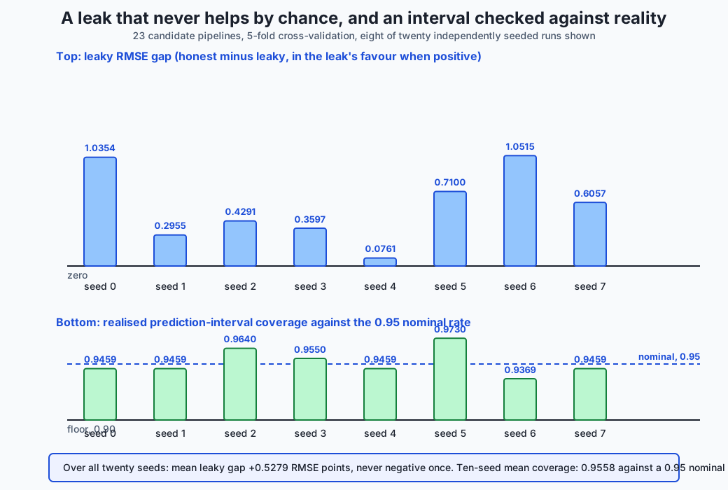
At the headline seed, the leaky search reports 55.5212 RMSE against the honest 56.5566 — a gap of 1.0354 points in the leak’s favour. Over 20 seeds, the mean gap is +0.5279 (standard deviation 0.3686, minimum 0.011, maximum 1.1451), and — the structural fact worth remembering — it is never negative, at any seed tried. The leaky search considers the honestly selected winner among its 23 candidates and can only replace it with something that scored at least as well (as low or lower RMSE) on the very rows it was allowed to peek at. It cannot report a worse number. It can only match or improve on the honest score, which is not luck — it is the mechanism.
Prediction intervals, and their realised coverage
A point prediction alone is not a complete answer — “56.5566 RMSE” tells
you about average error, not about the range any individual prediction
might plausibly be wrong by. A prediction interval addresses that, and
this lesson builds one the honest way: from training out-of-fold
residuals only, via cross_val_predict, never from the test residuals
themselves — sizing an interval from the same data it is checked against
would be circular, the same discipline error GatedTestSet exists to
prevent.
95 percent prediction interval half-width (from TRAIN out-of-fold residuals): +/-105.8797
realised coverage on the 111 test rows: 0.9459  (nominal: 0.9500)
0.9459 against a stated 0.95 is close — a prediction interval whose nominal rate roughly matches what actually happens, checked rather than assumed. A separate ten-seed measurement (not part of the harness’s asserted claims, reported here for context) gives a mean coverage of 0.9558, ranging from 0.9369 to 0.9910 — consistently near the nominal rate, with the ordinary scatter you would expect on a test set this small.
An everyday analogy
A home inspector examining a house before sale.
Baseline is what you’d predict about any house’s condition knowing nothing but the neighbourhood average sale price adjusted for square footage — the number your specific inspection has to beat to be worth paying for.
The frame is deciding, precisely, what you are assessing: not “is this a good house” but “what is this specific house’s likely repair cost, based on this specific inspection.”
The split is deciding, before entering the house, which rooms and systems inform the written report (every room, every visible system, looked at as many times as needed) and which single test is held back for a final, one-time check — say, a water-pressure test run once, at the very end, purely to confirm nothing was missed.
The sweep is trying several different weighting schemes for combining observations into a repair-cost estimate — weight the roof heavily, weight the foundation heavily, weight the electrical system heavily — and scoring each scheme against past inspected houses whose actual repair costs are already known.
Cross-validation is checking each weighting scheme against several different subsets of those past houses, not just one, so a scheme that happened to work on one arbitrary batch of history does not get crowned the winner by luck.
Selection is the inspector settling on one scheme — the one that predicted past repair costs most accurately, on average, across those checks.
The one look is applying that agreed-upon scheme to the actual house being inspected today, once, and writing the number down. Not re-weighting after peeking at what the final number “would have been” under five different schemes and quietly picking whichever gives the number the seller wants to see.
Residual diagnostics is the inspector who, instead of reporting only “estimated repair cost: $8,400,” goes back through every past house where the estimate was wrong and checks: were the misses bigger on expensive houses than cheap ones? Did the errors cluster around a specific type of house? Were the five worst misses all the same kind of mistake, or five different kinds? An inspector who reports the average error and stops has told you less than one who tells you where the estimate tends to fail.
The fairness check is asking, specifically: are inspection estimates systematically less accurate for the most expensive, most severely damaged houses — the ones where an accurate number matters most to someone deciding whether to buy?
Prediction intervals are the inspector who says “$8,400, plus or minus $2,100” instead of a bare number — and then, crucially, checks their own track record: across the last hundred houses where they gave a range, did the true repair cost actually fall inside that range roughly 95 percent of the time, as claimed? An inspector whose “95 percent” ranges are only right 70 percent of the time has a miscalibrated instrument, and the only way to find that out is to check.
The verdict is not “the house checks out.” It is “here is the estimate, here is the honest range around it, here is where the estimate tends to be wrong, and here is whether this specific house’s estimate clears the noise level given how many past houses this scheme was checked against.”
The analogy earns its keep on the leaky-selection failure. Imagine an inspector who, instead of trusting the pre-agreed weighting scheme, quietly tries all twenty-three schemes on this specific house, compares each one’s estimate against a quick informal peek at what the seller’s own contractor quoted, and reports whichever scheme’s estimate was closest — then writes it up as though it were the pre-agreed process’s output. That report can never look worse than the honest process would have; at absolute worst it ties. The dishonesty is invisible in the number itself; it lives entirely in which of twenty-three schemes got reported after the fact.
Examples in practice
A learner who reports RMSE and stops
The most common mistake this lesson is built to correct: a project that reports “56.5566 RMSE” and nothing else. Three follow-up questions immediately matter, none of them answered by the headline number alone. 56.5566 compared to what — a baseline of 70.4637, where the same number would mean real progress, or a baseline of 58, where it would mean almost nothing? What do the residuals look like — flat and normal, or fanning out and skewed? And is the model’s error worse for the cases that matter most — here, patients with more severe progression? All three questions have concrete, measured answers in this lesson, and none is visible in 56.5566 by itself.
A team that tunes against its own held-out set without noticing
The most common real instance of the leaky-selection mistake rarely
looks like a single dramatic error. It looks like a team with one
official test set that tries a model, checks the test RMSE “just to
confirm,” tries a hyperparameter tweak, checks again, tries a different
feature transform, checks again — and after the fifth check, reports the
best-scoring version as “our result.” No single check felt like
cheating. The cumulative effect is exactly leaky_selection_test_rmse: K
looks at the test set disguised as one, and the reported number can only
ever look as good or better than an honest single look, never worse. The
fix is not vigilance — it is a GatedTestSet that makes the sixth look
impossible rather than merely inadvisable.
A model comparison that never checks its own margin against an interval
An analyst is asked whether a new pricing model beats the old one by 3 RMSE points. Before touching any code: on a test set of 111 rows, resolving that comparison with confidence requires knowing the noise floor a bootstrap of that size would produce — this lesson’s own margin interval, [5.5852, 22.3324] around a 13.9071-point margin, has a half-width around 8.4 points. A claimed 3-point improvement on a similarly small test set would very likely be swallowed by that same noise, and the honest answer would be “this comparison cannot be made with the data available,” delivered before a single model is retrained.
Reading a published model’s headline RMSE without the residuals
A vendor reports “our model achieves 12 percent lower RMSE than the baseline.” The number alone answers almost nothing about whether the model is trustworthy in practice. Are the errors evenly spread, or does the model have a handful of catastrophic misses concentrated in one subgroup — exactly the pattern today’s largest-residuals check and fairness-by-target-level check are built to surface? A model that is excellent on average while being reliably, severely wrong on a specific category of case can post an impressive headline RMSE while being far less trustworthy than the number alone suggests.
Implications: security, privacy, performance, scalability, and cost
The cost of skipping a baseline is a project that never gets challenged. A model reporting 68 RMSE on data where the mean-predictor baseline is 70.4637 will pass every casual review, because 68 sounds like an improvement. The baseline is a one-line, zero-cost check that catches this before anyone spends a week building on top of it.
The cost of a leaky selection is a number that fails in production and
nowhere else. Every metric a team reports internally can look
consistent right up until deployment, because the leak lives entirely in
how the number was produced, not in any property of the data a dashboard
could flag. GatedTestSet is a cheap, mechanical defence against exactly
this — one object, refusing a second call, costs nothing to add and
closes the most common real-world version of this mistake.
Residual diagnostics are a reliability control, not a nicety. A model whose errors fan out with the prediction size (a positive heteroscedasticity signal, as measured here) will be systematically overconfident on its largest predictions if that signal is ignored — and a downstream system that treats every prediction as equally reliable inherits that overconfidence silently.
A fairness check on error by target level is a safety control in any domain where the target correlates with stakes. On a disease- progression score, a model systematically worse for more severe cases would be worse exactly where accuracy matters most. This lesson’s measured result — nearly flat, 1.0473 — is reassuring, but only because the check ran; an unchecked model provides no such reassurance by default.
Computing a bootstrap interval costs 2000 extra RMSE calculations on a test set that is already small — cheap here, and cheap on almost any dataset this size. The trade-off Day 144 named for accuracy intervals applies identically here: on a real project of this scale, skipping the interval to save compute is never the right call.
And the largest, least visible cost is a project that never runs the residual diagnostics because “the RMSE already looked fine.” This lesson’s own result — a modest but real heteroscedasticity signal, a near-flat but genuinely measured fairness check, a prediction interval whose coverage had to be checked rather than assumed — is the argument for running the full protocol, not evidence that any of it was unnecessary because nothing came back alarming.
Alternatives: free, open source, and commercial
scikit-learn’s own regression and selection tools — used throughout this lesson
When to choose them: for essentially all in-memory regression work.
Every stage of today’s protocol — Pipeline, KFold, cross_val_score,
cross_val_predict, DummyRegressor — is free, BSD-3-Clause licensed,
with no paid tier, and every number in this lesson comes from them.
How to use them: chained together exactly as shown in “How it
works” — a Pipeline per candidate, cross_val_score for the sweep,
cross_val_predict for out-of-fold residuals, and hand-rolled bootstrap
and residual-diagnostic functions, since scikit-learn does not ship an
interval helper for RMSE or a Q-Q correlation directly.
Watch for: Pipeline protects you from leaking a fitted transform
across the train/test boundary, but it does not protect you from leaking
the test set itself into selection — this lesson’s leaky-selection
exercise happens entirely outside any estimator’s contract, in how you
choose to call .score() or .predict().
statsmodels — described, not used here
When to choose it: when you need classical inferential statistics
alongside prediction — p-values, confidence intervals on individual
coefficients, formal heteroscedasticity tests like Breusch-Pagan, or
residual diagnostic plots built in. statsmodels’s OLS class returns a
results object with .summary(), giving a full classical regression
table scikit-learn intentionally omits.
What it adds: built-in statistical tests this lesson’s correlation-based signals approximate by hand — a formal Breusch-Pagan test for heteroscedasticity, a Jarque-Bera test for normality, rather than the correlation-based approximations this lesson builds to avoid a scipy dependency.
Honest note: this lab is not installed with statsmodels and no
output from it is reproduced anywhere in this lesson. The residual
diagnostics here are hand-built specifically to work with only the three
pinned packages (numpy, scikit-learn, pytest); a project already
using statsmodels would reasonably prefer its formal tests over this
lesson’s correlation-based signals.
scipy.stats — described, not used here
When to choose it: for a proper Q-Q plot (scipy.stats.probplot), a
formal Shapiro-Wilk normality test, or a closed-form confidence interval
on RMSE derived from the chi-squared distribution of squared residuals
under a normality assumption.
What it costs: nothing — free, BSD-licensed, and already installed as a scikit-learn dependency on most systems, though not one this lab imports directly.
Honest note: this lesson builds its own normal-probability
correlation from scratch — a rational approximation to the inverse
normal CDF — specifically so the lab’s three pinned dependencies
(numpy, scikit-learn, pytest) stay sufficient. Day 153’s habit,
applied again: build the minimal piece you need rather than reach past
the pins.
Managed experiment-tracking and model-monitoring platforms — not used here
The relevant capability for this lesson: automatic residual dashboards and drift monitoring that would compute today’s heteroscedasticity and fairness-by-target-level checks continuously in production, rather than once at project time.
Free versus paid: most offer a free tier for individual use and charge for team or production features; no specific price is quoted here, because pricing changes faster than this lesson does, and an unverified figure is worse than none. Free, self-hosted, open-source options exist and can compute the same diagnostics this lesson builds by hand.
Comparison with related concepts
| Concept | What it does | How it relates to today |
|---|---|---|
| A single train/test split | one division, one score | What this lesson’s split stage builds on, and what cross-validation replaces for selection |
| Cross-validation | every training row tests exactly once | Used here to select among 23 candidates without ever touching test rows |
| Bootstrap interval on a margin | resamples the test set to size uncertainty around a difference | This lesson’s verdict machinery, extending Day 144’s accuracy interval to RMSE, which has no equally simple closed form |
| Residual-vs-fitted diagnostics | reads the pattern in errors, not just their summary | This lesson’s centrepiece; owned by no earlier day in this course |
| Q-Q / normal-probability check | tests whether residuals are shaped like a bell curve | Built from scratch here without scipy; scores 0.9901, close to normal |
| Error by target level | RMSE split by a covariate of interest | This lesson’s fairness check; came back nearly flat, a real and valuable finding |
| Leaky selection | choosing a model by scoring it on the test set | Deliberately reconstructed in exercise 10, for regression, mirroring Day 147’s classification version |
| GatedTestSet | mechanically enforces one test evaluation | Reused unchanged from Day 144 and Day 147, protecting the real test rows of a real regression project |
| Prediction interval, with measured coverage | a range around a prediction, checked against reality | This lesson’s own interval, sized from training residuals only, checked at 0.9459 against a 0.95 nominal rate |
Two rows deserve a closing note.
The residual-diagnostics row is this whole lesson’s reason for existing. No earlier day in this course stops to read what the errors themselves look like rather than summarising them into one number. Every other row in this table has an earlier-day counterpart; this one does not, and it is deliberately the section this lesson spends the most attention on.
And the leaky-selection row is the mistake most likely to happen to
you specifically, more than group leakage or temporal leakage, because
it requires no unusual data structure — just checking the test score one
extra time. GatedTestSet exists because good intentions are not a
reliable enough defence against a mistake this easy to make by accident,
in regression exactly as much as in classification.
When to use it — and when not to
Run the full protocol whenever a regression result will inform a real decision — a deployment, a publication, a pricing model someone will act on. The cost is an afternoon and a handful of extra function calls; the alternative cost, when this protocol is skipped, is a number that fails exactly when it matters most.
Compute the residual diagnostics on every real regression project, not only when you suspect a problem. This lesson’s own result — real but modest signals, neither dismissed nor treated as a crisis — was only knowable because the check ran.
Open the fairness-by-target-level check whenever the target correlates with real-world stakes, which is most regression problems worth building. A flat overall RMSE can hide a model that is systematically worse exactly where accuracy matters most.
Compute the bootstrap interval around any claimed margin before treating a model comparison as settled. An improvement smaller than the interval’s half-width is not evidence of anything, however good the point estimate looks.
Check the realised coverage of any prediction interval you report. A “95 percent interval” that has never been checked against reality is a claim, not a measurement.
And use GatedTestSet, or an equivalent, whenever more than one
person or more than one script can reach the test set — the
leaky-selection mistake this lesson reconstructs almost never happens on
purpose.
When the full protocol is more than the situation needs: a genuinely exploratory first look at brand-new data, where nothing will be reported or deployed and the goal is purely to build intuition, can reasonably skip the formal split-and-gate machinery — provided nobody later reuses that exploratory number as though it were a validated result. The moment a number leaves the exploratory phase and starts informing a decision, the full protocol applies.
The AI thread
Every stage of today’s protocol gets harder, not easier, at the scale modern AI systems operate at, and the residual-diagnostics finding is the sharpest version of why.
A large model’s “residuals” are almost never inspected at the level of individual failures the way today’s five worst mistakes were. A language model evaluated on an aggregate score — perplexity, an average human-preference rating, a benchmark accuracy — can carry the exact regression-diagnostics failure this lesson measured: a model that looks excellent on average while being reliably, severely wrong on a specific, identifiable category of input. Today’s discipline — read the worst individual mistakes by name, not just the summary statistic — is exactly what a responsible evaluation of a much larger system still requires, and it is far more often skipped at that scale than at this one, because there is no equivalent of “print the five worst rows” for a system processing millions of interactions without deliberate sampling.
The fairness-by-target-level check has a direct, higher-stakes analogue in AI evaluation. This lesson asked whether errors were worse for patients with more severe disease progression — the group where accuracy plausibly matters most. The same question, asked of a language model, becomes: is the system systematically less reliable for the users, languages, or use cases where a mistake would be most costly? A model with an excellent aggregate score and a specific, unmeasured subgroup where it fails badly is not a hypothetical — it is the most common way an aggregate evaluation misleads, and this lesson’s flat 1.0473 result is a reminder that the check sometimes comes back reassuring too; the point is that you cannot know which case you are in without running it.
And prediction intervals with checked coverage are the honest alternative to a model that reports only a point estimate with false confidence. A large language model producing a single “best” answer, with no calibrated sense of its own uncertainty, is the aggregate-scale version of a regression model reporting 56.5566 RMSE with no interval attached. The discipline this lesson teaches at the scale of 111 test rows and one prediction interval — build the range from held-out data, then measure whether reality actually falls inside it as often as claimed — is the same discipline a trustworthy AI system needs at any scale, and it is measured far less often than the raw accuracy number that gets the headline.
Knowledge check
candidate_summaries(via exercise 1’s assertions) confirmsload_diabetesneeds no download whilefetch_california_housingdoes. Name the specific attribute checked, and explain why this lesson treats it as disqualifying rather than merely inconvenient.- Plain OLS scores 54.0926 cross-validated RMSE, only 0.1968 points
behind the winning
Lasso(alpha=1)at 53.8958 — yet Day 150 measured severe multicollinearity (VIFs up to 59.2) on these exact features. Explain how both facts can be true at once. - The margin over baseline is 13.9071 RMSE points, and its 95 percent bootstrap interval is [5.5852, 22.3324]. State the rule connecting these two numbers to the verdict, and describe a hypothetical margin size that would have forced a “cannot distinguish” verdict instead.
- The heteroscedasticity signal is 0.2386 and the curvature signal is -0.1278. Explain what each one measures, and why neither value alone justifies calling this model’s residuals either “perfectly well-behaved” or “seriously flawed.”
- The fairness-by-target-level check gives a ratio of 1.0473. Explain why this near-flat result is still a valuable finding, rather than a sign the check was unnecessary.
- In the leaky-selection exercise, the RMSE gap is sometimes small (0.011) but never negative, across twenty seeds. Explain the mechanism that makes a negative gap impossible.
- The prediction interval’s half-width comes from training out-of-fold residuals, never from the test residuals. Explain what would go wrong if the test residuals were used instead, and connect it to a pattern from an earlier day in this course.
- State, in order, the stages of this lesson’s protocol, and name one specific measured failure from Days 148-153 or Day 144/147 that each stage defends against.
Hands-on exercise
Today’s lab, A Complete Regression Project, runs the entire protocol
on the diabetes-progression dataset and asks you to verify every
measured number along the way.
Fourteen exercises. The first four establish the dataset choice, the baseline, the split and the sweep. The next three build the cross-validated selection, the gated one-time test evaluation, and the bootstrap interval around the margin. The next three cover residual diagnostics — the centrepiece — and the fairness check by target level. The last four cover the leaky-selection reconstruction and the prediction interval’s realised coverage.
Build the environment, then work through
starter/test_regression_claims.py, replacing one pytest.skip at a
time.
Expected output
The harness ends with:
---------------------------------------------------------------
15 checks, 0 failure(s)
and exits 0. pytest examples -q reports 19 passed, and
pytest starter -q reports 5 passed, 14 skipped until you begin.
The measured table includes:
  K = 23 candidate pipelines: 11 ridge, 11 lasso, 1 plain OLS
  winner: lasso (alpha=1)  5-fold CV RMSE = 53.8958
  test RMSE: 56.5566  R2: 0.3557  MAE: 45.2846
  margin (baseline RMSE - model RMSE): +13.9071
  95 percent bootstrap interval on the margin: [5.5852, 22.3324]
  heteroscedasticity signal, corr(fitted, |residual|): +0.2386
  curvature signal, corr(fitted^2, residual): -0.1278
  normal-probability (Q-Q) correlation: 0.9901
  RMSE on below-median targets: 55.2464   above-median: 57.8601   ratio: 1.0473
  mean leaky gap: +0.5279  sd 0.3686  min +0.0110  max +1.1451
  95 percent prediction interval half-width: +/-105.8797  realised coverage: 0.9459
Validate your work
bash tests/run_tests.sh; echo "exit=$?"reports15 checks, 0 failure(s)andexit=0. Capture the harness’s own exit status..venv/bin/pytest examples -qreports19 passed..venv/bin/python3 examples/report_measurements.py | diff - expected-output/measured-values.txtproduces no output.- When you have finished every exercise,
pytest starter -qreports19 passed. - Break one assertion on purpose, confirm the harness fails, restore it.
Troubleshooting
My winning configuration differs from the lesson’s. Check
expected-output/FIELDS.md. Several configurations score within two
tenths of a point of Lasso(alpha=1), and different NumPy or scikit-learn
versions can legitimately shuffle a near-tie differently — Day 145
already established that near-tied configurations trade places under
resampling.
The bootstrap interval doesn’t match my by-hand calculation.
margin_bootstrap_interval seeds its own random generator internally
(default seed=0); calling it with different arguments, or a different
n_boot, will legitimately produce different bounds.
My leaky-gap numbers differ from the lesson’s. Almost certainly fine at the level of the decimals. What must hold across the full 20-seed sweep is that the gap is never negative.
import file mismatch. You ran pytest examples starter together.
Run them separately.
Common mistakes
Reporting the test RMSE without the margin interval. A point estimate with no half-width is not a verdict, and this lesson’s own comparison — 13.9071 improvement against an interval half-width around 8.4 points — would have looked very different at a smaller improvement or a smaller test set.
Treating the modest residual-diagnostic signals as either “nothing” or “a crisis.” Neither reading matches what was actually measured: real, non-zero, and not dramatic.
Sizing a prediction interval from the test residuals themselves.
This is circular — using the answer to size the check against that same
answer — and it is the same discipline error GatedTestSet exists to
prevent for point predictions.
Concluding the leaky-selection gap is “basically zero and therefore harmless” because some seeds are small. The gap’s size varies, but it is never negative across twenty seeds — the mechanism, not the size, is the point.
Practice assignment
Take a regression result you already have — from a project, a tutorial, or your own experiments — and run this lesson’s protocol against it, honestly.
- State your baseline. What does predicting the mean get you for free? If you cannot answer this in one line, your project has not been framed yet.
- Count your K. How many models or hyperparameter settings were tried against whatever number you are about to report? Estimate it honestly, in writing, even if the true count is embarrassing.
- Compute a margin interval, using a bootstrap over your own test set, and compare it to whatever improvement you are claiming.
- Read your residuals. Plot or compute the heteroscedasticity and curvature signals this lesson built, and name the five largest individual mistakes your model makes.
- Check whether your errors are worse for a specific group that matters in your domain — not just which group is more frequent, but which group’s accuracy carries the highest real-world stakes.
- If you report a prediction interval, check its realised coverage against its nominal rate. If you have never checked this, say so plainly — that is a finding too.
The deliverable is the audit, in writing, not a better model.
Extension challenge
Pick one and measure it.
- Nested cross-validation. Implement an inner selection loop and an outer scoring loop, and measure whether the gap between cv_rmse and the outer-scored RMSE shrinks further than this lesson’s single test evaluation showed. Report the cost in fits.
- A fourth candidate family. Add
ElasticNetto the sweep, re-run the full protocol, and report whether the winner or its cross-validated RMSE changes at the headline seed. - Quartile-level fairness. Split the test set into quartiles rather than halves and determine whether the fairness-by-target-level signal strengthens toward the extremes rather than staying flat.
- Scale the test set and re-measure the leaky gap. Repeat the leaky-vs-honest comparison with a 60/40 train/test split instead of 75/25, so the test set holds roughly 177 rows instead of 111, and report whether the mean gap and its granularity both change.
- A per-row prediction interval. Build a version whose half-width varies with the fitted value, rather than staying constant, and compare its coverage and average width to this lesson’s constant-width version.
- Break independence on purpose. Duplicate a fraction of the rows into both the train and test splits before running the sweep, and measure how much the reported test RMSE improves (misleadingly) — Day 144’s group-leakage lesson, reconstructed on real regression data.
Quiz
Q1. This lesson uses sklearn.datasets.load_diabetes(scaled=False) rather than fetch_california_housing, even though the latter is a larger, more well-known regression dataset. Why, specifically?
- fetch_california_housing downloads its data on first use (download_if_missing defaults to True), which this lab's offline rule forbids; load_diabetes is bundled inside scikit-learn itself
- load_diabetes has more rows than fetch_california_housing
- fetch_california_housing only supports classification, not regression
- load_diabetes is the only regression dataset with a physical unit on its target
Show answer
Answer: A. fetch_california_housing downloads its data on first use (download_if_missing defaults to True), which this lab's offline rule forbids; load_diabetes is bundled inside scikit-learn itself
inspect.signature(fetch_california_housing).parameters['download_if_missing'].default is True -- confirmed directly in exercise 1 -- which makes it network-dependent and therefore forbidden by this lab's safety rule (A37). load_diabetes ships as bundled arrays inside the installed scikit-learn package and needs no network at all. The row-count and classification claims are both false: fetch_california_housing has more rows, and both datasets are regression problems. The unit claim is also false in the other direction -- this lesson's target has NO physical unit, and that is stated plainly rather than invented.
Q2. The mean-predictor baseline on the test set scores 70.4637 RMSE and an R2 of -0.0001. What does the R2 close to zero (rather than exactly zero) tell you?
- That the baseline model is broken and should be debugged
- That the test set's mean target value is very close to, but not identical to, the training set's mean -- R2 of exactly 0.0 only holds when a model predicts the training mean and is scored against data with that exact same mean
- That RMSE and R2 are inconsistent metrics and one of them must be wrong
- That the dataset has too few rows to compute R2 reliably
Show answer
Answer: B. That the test set's mean target value is very close to, but not identical to, the training set's mean -- R2 of exactly 0.0 only holds when a model predicts the training mean and is scored against data with that exact same mean
DummyRegressor(strategy='mean') predicts the TRAINING mean for every row. R2 is defined relative to the mean of whatever it is scored against -- here, the TEST set's mean, which differs very slightly from the training mean because of the random split. That tiny difference is exactly what produces an R2 of -0.0001 instead of a perfect 0.0. Nothing is broken, and RMSE and R2 are simply two different formulas computed from the same residuals -- they do not need to "agree" in any stronger sense than that.
Q3. Plain OLS scores 54.0926 cross-validated RMSE at seed 0, only 0.1968 points behind the winning Lasso(alpha=1) at 53.8958 -- yet Day 150 measured VIFs as high as 59.2 on this exact dataset's raw features. How should these two facts be read together?
- They contradict each other, so one of the two measurements must be wrong
- Multicollinearity always makes predictions worse, so the small gap here is a bug
- Multicollinearity destabilises the individual COEFFICIENTS (Day 150's finding) without necessarily destabilising PREDICTION accuracy by very much -- regularisation's benefit here is real but modest, which this lesson measures rather than assumes
- The VIF measurement from Day 150 is irrelevant to regression entirely
Show answer
Answer: C. Multicollinearity destabilises the individual COEFFICIENTS (Day 150's finding) without necessarily destabilising PREDICTION accuracy by very much -- regularisation's benefit here is real but modest, which this lesson measures rather than assumes
Day 150's finding was specifically about coefficient instability under correlated predictors, not about prediction accuracy. A model can have wildly unstable individual coefficients while still producing nearly-as-good predictions as a regularised alternative, because the correlated predictors can substitute for one another in the fitted equation even as their individual weights swing. This lesson measures the prediction-accuracy gap directly (0.1968 RMSE points) rather than assuming regularisation must produce a dramatic improvement just because multicollinearity is present.
Q4. The winning model's margin over baseline is 13.9071 RMSE points. A 2000-draw bootstrap gives a 95 percent interval on that margin of [5.5852, 22.3324]. What is the correct verdict?
- Cannot distinguish the model from the baseline, because the interval is wide
- The model overfit, because the margin is large relative to the baseline
- No verdict is possible until the test set is evaluated a second time to narrow the interval
- The margin is distinguishable from zero, since the interval's lower bound (5.5852) is comfortably positive -- the model beats the baseline by more than sampling noise on 111 test rows could plausibly explain
Show answer
Answer: D. The margin is distinguishable from zero, since the interval's lower bound (5.5852) is comfortably positive -- the model beats the baseline by more than sampling noise on 111 test rows could plausibly explain
The interval excludes zero entirely -- its lower bound is 5.5852, well above zero -- so the improvement is distinguishable from baseline at this test-set size, even though the interval itself is wide (as expected on only 111 test rows). Interval width alone does not determine the verdict; whether the interval excludes zero (or, more generally, whatever threshold defines "no improvement") does. A second test evaluation would not narrow anything -- per Day 144's GatedTestSet discipline, it would produce a validation score wearing the word test. And a large margin over baseline says nothing about overfitting without comparing train and validation behaviour, which Day 145 covered separately.
Q5. The heteroscedasticity signal (correlation of fitted value with absolute residual) is 0.2386, and the curvature signal (correlation of squared fitted value with signed residual) is -0.1278. How should a reader interpret these two numbers together?
- Both signals are real but modest -- a mild tendency for errors to grow with the prediction, and a weak, inconclusive hint of a missed curve -- worth reporting honestly rather than either dismissed or treated as alarming
- Both signals indicate the model is badly overfit and must be discarded
- A positive heteroscedasticity signal always means the model is unusable for prediction
- These two numbers should be identical if the residuals are well-behaved, so their difference is an error
Show answer
Answer: A. Both signals are real but modest -- a mild tendency for errors to grow with the prediction, and a weak, inconclusive hint of a missed curve -- worth reporting honestly rather than either dismissed or treated as alarming
Neither 0.2386 nor -0.1278 is close to the extremes (near +/-1) that would indicate a dramatic, unmissable pattern in a residual-vs-fitted plot. They are genuine, real signals -- not exactly zero -- but modest enough that this lesson reports them as "worth watching, not alarming" rather than either direction of overstatement. The two correlations measure different things (error MAGNITUDE growing with fitted value, versus a systematic CURVE in signed error) and have no reason to be equal or even similar in size.
Q6. Error by target level gives RMSE 55.2464 on the below-median half of test targets and 57.8601 on the above-median half -- a ratio of 1.0473. What is the honest reading of this result?
- The check was a waste of time, since the ratio came out close to 1.0
- A ratio close to 1.0 means this specific measured run found only a small (4.73 percent) difference in error between severity levels -- a real, if modest, finding that had to be measured rather than assumed, and a different seed or a different dataset could easily show a larger asymmetry
- The model must be discarded because it treats every target value identically
- A ratio close to 1.0 proves the model is fair on every possible fairness definition
Show answer
Answer: B. A ratio close to 1.0 means this specific measured run found only a small (4.73 percent) difference in error between severity levels -- a real, if modest, finding that had to be measured rather than assumed, and a different seed or a different dataset could easily show a larger asymmetry
Measuring this and finding it nearly flat is still valuable information -- the alternative, skipping the check because "it probably doesn't matter," would have left a real fairness-relevant question unanswered. A ratio of exactly 1.0 is not achieved (it is 1.0473, not 1.0000), so the model does not treat every value identically; the difference is simply small at this seed on this dataset. Nothing about one ratio close to 1.0 generalises to "fair on every definition" -- it answers only the specific question this check asks (RMSE by severity half), not every possible fairness question.
Q7. Exercise 10 selects a model by fitting all 23 candidates and scoring each one directly on the test set (keeping the lowest RMSE), instead of selecting on cross-validated training rows. Over 20 seeds, this leaky RMSE is never higher than the honest RMSE. Why can the leaky RMSE never come out worse?
- Because the leaky search always uses more training data than the honest one
- Because the leaky search considers the honestly selected winner among its 23 candidates, and can only replace it with something that scored at least as well (as low or lower RMSE) on the very test rows it was allowed to peek at
- Because ridge regression always outperforms lasso on this dataset
- Because the test set is larger than the training set in this lesson
Show answer
Answer: C. Because ridge regression always outperforms lasso on this dataset
The leaky search is a superset of the honest choice: it evaluates every one of the 23 candidates, including whichever one cross-validation selected, directly against the test rows, and keeps whichever produces the lowest RMSE on those same rows. By construction it therefore cannot report a HIGHER (worse) RMSE than the honestly selected model's own test score -- it can only match or beat it, which is the exact mechanism, not chance. Training-set size is identical between the two searches, and no single family (ridge, lasso, or OLS) systematically wins across all 20 seeds.
Q8. A prediction interval is built with a constant half-width of 105.8797, derived from the standard deviation of out-of-fold residuals on the TRAINING rows. Its realised coverage on the 111 test rows is 0.9459, against a stated (nominal) rate of 0.95. What would have been wrong about sizing this interval from the TEST residuals instead?
- Nothing -- test residuals would have given a more accurate interval
- Test residuals are always larger than training residuals, so the interval would have been too wide
- Using the test residuals to size an interval that is then checked for coverage on those same test residuals is circular -- it would inflate the apparent accuracy of the interval using information the interval is supposed to be evaluated against, the same discipline error Day 144 built GatedTestSet to prevent
- Test residuals cannot be computed at all, since the model was never evaluated on the test set
Show answer
Answer: C. Using the test residuals to size an interval that is then checked for coverage on those same test residuals is circular -- it would inflate the apparent accuracy of the interval using information the interval is supposed to be evaluated against, the same discipline error Day 144 built GatedTestSet to prevent
Sizing an interval from the very data used to check its coverage is a leak in exactly the shape Day 144 and Day 147 both taught: any quantity derived from test data and then evaluated against that same test data is contaminated, because it has seen the answer it is being scored against. Training out-of-fold residuals (via cross_val_predict) never touch the test rows, so the coverage check that follows is honest. Test residuals ARE computable (the model was in fact evaluated once, through the gate), which makes option D factually wrong, and there is no general rule that test residuals are always larger.
Glossary
- Mean-predictor baseline
- The RMSE and R2 of predicting the training mean for every test row, with no model at all. Every model in this lesson has to clear it to be worth building -- here, 70.4637 RMSE -- and it is computed before any model is fitted, not after, as a check on whether the whole exercise is worth doing.
- Candidate pipeline
- One complete, fittable scikit-learn Pipeline -- a specific estimator with specific hyperparameters, any preprocessing folded in. This lesson sweeps 23 of them: 11 ridge regularisation strengths, 11 lasso regularisation strengths, and 1 plain OLS.
- K, counted
- The number of candidates actually tried in a selection sweep. Day 144 named it as the number nobody remembers; this lesson counts it explicitly at 23, because a defensible model comparison needs it stated, not estimated.
- 5-fold cross-validation, scored by RMSE
- Splitting the training rows into five folds and scoring every candidate on all five, so every training row serves as held-out data exactly once. The scoring metric -- RMSE -- is chosen before any candidate is fitted, in the target's own unitless composite-score points.
- The margin
- The improvement of a winning model's test RMSE over the baseline RMSE. Here, 70.4637 minus 56.5566 equals 13.9071 RMSE points -- the number a bootstrap interval is computed around, not trusted on its own.
- Bootstrap interval on the margin
- A 95 percent interval built by resampling the test rows with replacement thousands of times and recomputing both RMSEs on each resample. Computed here as [5.5852, 22.3324] -- since it excludes zero, the model is distinguishable from baseline at this test-set size.
- GatedTestSet
- An object that wraps the held-out test rows and permits exactly one call to evaluate, raising TestSetTouchedTwice on any further attempt without advancing its own counter. The discipline from Day 144 and Day 147, made mechanical again on a regression problem.
- Leaky selection
- Choosing a winning configuration by fitting every candidate and scoring each one directly against the test set, keeping the lowest RMSE, instead of selecting on cross-validated training rows. Measured here at a mean gap of +0.5279 RMSE points over 20 seeds, and never negative at any seed tried.
- Residual
- The true target value minus the model's prediction, for one row. This lesson's centrepiece: reading the full set of residuals for patterns, not summarising them into a single RMSE and stopping there.
- Heteroscedasticity signal
- The correlation between a model's fitted value and the absolute size of its residual. Near zero means errors do not systematically grow or shrink with the prediction; here, 0.2386 -- a mild fanning-out, not a dramatic one.
- Curvature signal
- The correlation between the squared fitted value and the signed residual, used here as a numeric stand-in for a missed non-linear trend a residual-vs-fitted plot would show as a curve. Measured at -0.1278 -- weak, no strong evidence of a missed curve.
- Normal-probability (Q-Q) correlation
- A from-scratch check correlating sorted, standardised residuals against the quantiles a perfectly normal distribution would produce. 1.0 is a straight line; this lesson measures 0.9901, close to normal even on 111 real test rows.
- Error by target level
- RMSE computed separately on the below-median and above-median halves of the true test targets, to check whether a model is systematically worse for higher-value cases -- a fairness-relevant question on a disease-progression score. Measured here as a ratio of 1.0473: only 4.73 percent worse on the more severe half.
- Prediction interval
- A range around a point prediction meant to contain the true value with some stated probability -- distinct from a confidence interval, which describes uncertainty about a parameter rather than about one future observation. Built here with a constant half-width of 105.8797 from training out-of-fold residuals.
- Realised coverage
- The fraction of test targets that actually fall inside a prediction interval, checked against the interval's nominal (stated) rate. Measured here at 0.9459 against a 0.95 nominal rate on 111 test rows.
- Verdict
- The end product of a properly run regression project: a test RMSE, a bootstrap interval around its margin over baseline, a statement of whether the margin clears that interval, residual diagnostics, a fairness check by target level, and a prediction interval with measured coverage -- not a single RMSE quoted alone.
- Out-of-fold residual
- A residual computed on a training row while that row was held out of the fold used to fit the model -- via cross_val_predict -- so the residual reflects genuine held-out error rather than a fitted value the model has already seen. Used here to size the prediction interval without touching test rows at all.
Sources and further reading
- Ridge -- scikit-learn API reference — scikit-learn developers (accessed 2026-08-27)
- Lasso -- scikit-learn API reference — scikit-learn developers (accessed 2026-08-27)
- DummyRegressor -- scikit-learn API reference, for baseline models — scikit-learn developers (accessed 2026-08-27)
- cross_val_predict -- scikit-learn API reference — scikit-learn developers (accessed 2026-08-27)
- load_diabetes -- scikit-learn API reference, the dataset used in this lesson — scikit-learn developers (accessed 2026-08-27)
- Metrics and scoring: quantifying the quality of predictions -- model evaluation guide — scikit-learn developers (accessed 2026-08-27)
- Q-Q plot — Wikipedia (accessed 2026-08-27)
- Heteroscedasticity — Wikipedia (accessed 2026-08-27)
- Prediction interval — Wikipedia (accessed 2026-08-27)
Kept in this browser, no account needed. Your progress page turns the whole record into one link you can bookmark or open on another device.