Machine Learning › Trees and Ensembles › Day 164
Day 164: Gradient Boosting
Master the mathematical theory and implementation of Gradient Boosting from first principles: why boosting builds models sequentially rather than in parallel, how functional gradient descent treats trees as steps in function space, how to derive pseudo-residuals for arbitrary loss functions, why shrinkage (learning rate) prevents overfitting, and how Newton-Raphson leaf updates power modern tabular classifiers.
Hands-on lab for this lesson
Lab files on GitHub: https://github.com/ai-roadmap-365/ai-roadmap-365.github.io/tree/main/labs/sections/machine-learning/day-164-gradient-boosting
- Get the hands-on files. Clone the labs repository once (you can reuse this clone for every lesson). This works on macOS, Linux, and Windows (PowerShell or WSL):
git clone https://github.com/ai-roadmap-365/ai-roadmap-365.github.io.git cd ai-roadmap-365.github.io - Open this lesson's lab. Move into the directory for this specific day. Every lab lives at the same predictable path — section / subsection / week / day:
cd labs/sections/machine-learning/day-164-gradient-boosting - Read the lab guide. Open `README.md` in that directory. It lists the exact commands, what each does, the expected output, and how to check your work — read it before running anything.
- Run it and check your work. Follow the README's "How to run" section: run the example first to see the finished result, then complete the numbered exercises in `starter/`, then run the tests. The tests pass (exit 0) only when your work is correct.
bash tests/run_tests.sh # or the test command named in the lab README
You can also open the lab as a local page (works offline, shows the file tree and expected output).
Learning objectives
By the end of this lesson you will be able to:
- Formulate the additive model framework F_M(x) = F_0(x) + sum eta * h_m(x)
- Explain functional gradient descent and derive pseudo-residuals as negative loss gradients
- Derive the Newton-Raphson leaf value adjustment formula for binary cross-entropy loss
- Implement complete Gradient Boosting Regressors and Classifiers from scratch in NumPy
- Analyze the role of shrinkage (learning rate eta) as a regularizer in stochastic gradient boosting
- Contrast boosting (bias reduction) with bagging (variance reduction)
- Diagnose overfitting dynamics in boosting and configure early stopping with validation loss
- Benchmark custom gradient boosting against scikit-learn GradientBoostingClassifier
Prerequisites
- Day 162 -- Decision Trees
- Day 163 -- Random Forests and Bagging
Why this matters
In Day 163, we mastered Random Forests: an ensemble that trains dozens of deep, high-variance decision trees independently in parallel, using bootstrap sampling and random feature subsets to decorrelate the trees and reduce variance.
While Random Forests are robust and require minimal tuning, they treat each tree as a standalone estimator that knows nothing about the mistakes made by other trees.
What if, instead of training independent trees in parallel, we trained trees sequentially, with each new tree specifically designed to correct the residual errors made by the collective ensemble so far?
This is the paradigm of Boosting, and its mathematical pinnacle is Gradient Boosting, formulated by Jerome H. Friedman in 2001.
Gradient Boosting frames machine learning as gradient descent in function space. Rather than optimizing a fixed parameter vector w, gradient boosting iteratively adds shallow decision trees that point along the negative gradient of any differentiable loss function.
Today, gradient boosted trees power modern search engines, high-frequency trading systems, fraud detection engines, and tabular Kaggle championship solutions. Understanding gradient boosting from first principles is the bridge from classic machine learning to industrial state-of-the-art predictive modeling.
The idea in plain language
Imagine a master artist painting a hyper-realistic portrait:
- The Base Sketch (
F_0): The artist begins by painting a broad, rough outline of the face. This initial base layer captures the overall shape, but misses fine details and makes errors. - The First Correction (
h_1): The artist examines the canvas, identifies the areas with the largest errors (the residuals), and takes a fine brush to paint a correction layer over the shadows. - The Second Correction (
h_2): Stepping back again, the artist inspects the remaining mistakes. The next layer corrects the highlights and skin texture. - Shrinkage (Learning Rate
eta): Crucially, the artist does not apply thick, heavy brushstrokes all at once. Instead, they apply delicate, translucent glazes (scaling each correction byeta = 0.1). This prevents a single over-correction from ruining the painting.
After 100 sequential correction layers, the final portrait F_M(x) = F_0(x) + sum eta * h_m(x) achieves breathtaking accuracy that no single rough sketch could ever match.
Historical background
The theoretical foundation of boosting originated in computational learning theory with Michael Kearns and Leslie Valiant (1988), who posed a fundamental question: “Can a set of weak learners (models that perform slightly better than random guessing) be combined into a single strong learner?”
In 1990, Robert Schapire proved mathematically that this is always possible.
In 1996, Yoav Freund and Robert Schapire introduced AdaBoost (Adaptive Boosting), which reweighted misclassified training samples after each iteration. AdaBoost won the prestigious Gödel Prize for its mathematical elegance.
However, AdaBoost was strictly tied to exponential loss and classification.
In 2001, Jerome H. Friedman published Greedy Function Approximation: A Gradient Boosting Machine. Friedman realized that boosting is actually gradient descent in function space, where the pseudo-residuals are negative gradients of arbitrary loss functions (Squared Error, Log-Loss, Huber Loss, Poisson Deviance). Friedman’s generalization unlocked gradient boosting for all machine learning tasks.
What it is — and what it is not
To reason about Gradient Boosting with mathematical precision, let us establish what it is and is not:
What it IS:
- A Sequential Additive Model:
F_M(x) = F_0(x) + sum_{m=1}^M eta * h_m(x), where each base learnerh_mis trained sequentially. - Functional Gradient Descent: It minimizes empirical loss
sum L(y_i, F(x_i))by fitting base trees to the negative gradient of the loss. - A Bias and Variance Reducer: Unlike Random Forests (which primarily reduce variance), boosting drives down both bias and variance simultaneously.
- A General Framework for Any Loss: It can optimize any differentiable loss function (classification, regression, ranking, survival analysis).
What it is NOT:
- Not Parallel Across Trees: Because tree
mrequires the residuals from treem-1, trees cannot be trained simultaneously in parallel (though individual split searches within a tree can be parallelized). - Not Immune to Overfitting: Unlike Random Forests (where adding trees is always safe), adding too many boosted trees or using an excessive learning rate WILL overfit the training set.
- Not Scale-Dependent: Like all tree models, boosted trees are scale-invariant and require no numerical feature normalization.
Why it was created and what problems it solves
Gradient Boosting solves four fundamental challenges in competitive machine learning:
- Reaches the Theoretical Limit of Tabular Accuracy: Consistently outperforms linear models, k-NN, SVMs, and standard Random Forests on structured tabular data.
- Optimizes Custom Business Loss Functions: Allows data scientists to plug in specialized losses (e.g. asymmetric quantile loss for supply chain inventory, Huber loss for outlier-heavy finance).
- Efficient Model Capacity Control: Shallow base learners (depth 3 to 6) keep individual tree complexity low, preventing local memorization.
- Adaptive Error Correction: Automatically concentrates learning capacity on hard-to-classify samples and subtle edge cases.
How it works
Let us formulate the complete mathematics of functional gradient descent, loss functions, pseudo-residuals, Newton-Raphson leaf updates, and shrinkage.
1. Functional Gradient Descent Formulation
Given a training dataset D = { (x_1, y_1), ..., (x_N, y_N) } and a differentiable loss function L(y, F(x)), our objective is to find a function F^*(x) minimizing the empirical risk:
J(F) = sum_{i=1}^N L(y_i, F(x_i))
In standard gradient descent over model parameters w in R^D, we update parameters along the negative gradient:
w_{m} = w_{m-1} - eta * nabla_w J(w_{m-1})
In Functional Gradient Descent, we view the model’s predictions F = (F(x_1), ..., F(x_N))^T in R^N as a vector in N-dimensional function space.
The negative gradient of the loss with respect to the prediction at sample i is the pseudo-residual:
r_{im} = - [ (partial L(y_i, F(x_i))) / (partial F(x_i)) ]_{F(x) = F_{m-1}(x)}
Because we want our model to generalize to unseen points x, we cannot simply adjust the vector F directly. Instead, we train a base regression tree h_m(x) to predict the pseudo-residuals r_{im} for all i in {1, ..., N}.
The model is updated additively:
F_m(x) = F_{m-1}(x) + eta * h_m(x)
Where eta in (0, 1] is the shrinkage parameter (learning rate).
2. Common Loss Functions and Their Pseudo-Residuals
A. Squared Error Loss (Regression)
L(y, F) = (1/2) * (y - F)^2
r_i = - (partial L / partial F) = - [ -(y_i - F(x_i)) ] = y_i - F(x_i)
Result: For squared error, the pseudo-residual is simply the standard arithmetic residual y_i - F_{m-1}(x_i).
B. Log-Loss / Binary Cross-Entropy (Classification)
Let y in {0, 1} and let F(x) be the raw log-odds prediction:
p(x) = sigmoid(F(x)) = 1 / (1 + exp(-F(x)))
The binary cross-entropy loss is:
L(y, F) = - [ y * log(p) + (1 - y) * log(1 - p) ]
= - y * F + log(1 + exp(F))
Taking the derivative with respect to raw score F:
(partial L / partial F) = - y + (exp(F) / (1 + exp(F))) = - y + p
Therefore, the negative gradient (pseudo-residual) is:
r_{im} = - (partial L / partial F) = y_i - p_{m-1}(x_i)
- If
y_i = 1andp_i = 0.8:r_i = 1.0 - 0.8 = +0.2(Small positive push). - If
y_i = 1andp_i = 0.1:r_i = 1.0 - 0.1 = +0.9(Huge positive push). - If
y_i = 0andp_i = 0.9:r_i = 0.0 - 0.9 = -0.9(Huge negative push).
3. Newton-Raphson Leaf Value Adjustment
When we fit a regression tree h_m to the pseudo-residuals r_{im}, the tree partitions feature space into J disjoint regions (leaf nodes) R_{1m}, ..., R_{Jm}.
In a standard regression tree, the leaf value is the simple average of the targets in that leaf. However, for non-linear losses like Log-Loss, a simple average of gradients does not minimize the loss.
We solve for the optimal leaf step gamma_{jm} that minimizes loss in region R_{jm}:
gamma_{jm} = argmin_gamma sum_{x_i in R_{jm}} L(y_i, F_{m-1}(x_i) + gamma)
Taking a second-order Taylor expansion (Newton-Raphson step):
gamma_{jm} approx - ( g_j / H_j ) = ( sum_{x_i in R_{jm}} r_{im} ) / ( sum_{x_i in R_{jm}} p_{im} * (1 - p_{im}) + eps )
Where:
- Numerator: Sum of first derivatives (pseudo-residuals).
- Denominator: Sum of second derivatives (Hessian / curvature:
p * (1 - p)).
This Newton-Raphson leaf adjustment gives Gradient Boosting its astonishing convergence speed and mathematical rigor.
4. Step-by-Step Gradient Boosting Algorithm
Algorithm: Gradient Boosting Classifier
1. Initialize F_0(x) with optimal constant log-odds:
   F_0(x) = log(p_bar / (1 - p_bar))  where p_bar = (1/N) * sum y_i

2. For m = 1 to M:
   a. Compute probabilities: p_i = sigmoid(F_{m-1}(x_i)) for all i
   b. Compute pseudo-residuals: r_i = y_i - p_i for all i
   c. Fit a shallow regression tree h_m(x) of depth 3 to targets r_i
   d. For each leaf j in tree h_m:
         Compute optimal leaf value:
         gamma_j = sum_{i in Leaf_j} r_i / ( sum_{i in Leaf_j} p_i * (1 - p_i) + 1e-15 )
   e. Update model:
         F_m(x) = F_{m-1}(x) + eta * sum_j gamma_j * I(x in Leaf_j)

3. Final Probability Output:
   p(x) = sigmoid(F_M(x)) = 1 / (1 + exp(-F_M(x)))
An everyday analogy
Think of Gradient Boosting as an Olympic archery coach:
- Round 0 (
F_0): The archer aims directly at the center of the target. The arrow lands 4 inches high and 2 inches to the right (Residual =[-4, -2]). - Round 1 (
h_1): The coach instructs: “Compensate by aiming 0.4 inches lower and 0.2 inches left” (Shrinkageeta = 0.1). The archer shoots again. Now the arrow is only 1 inch high. - Round 2 (
h_2): The coach calculates the new residual and advises a micro-adjustment of 0.1 inches lower. - The Over-Coaching Danger (Overfitting): If the coach provides 5,000 micro-adjustments, the archer will begin compensating for a momentary gust of wind that happened 20 minutes ago. The archer memorizes random gusts rather than learning true shooting technique.
Examples in practice
Let us visualize the complete Gradient Boosting additive pipeline and pseudo-residual flow:
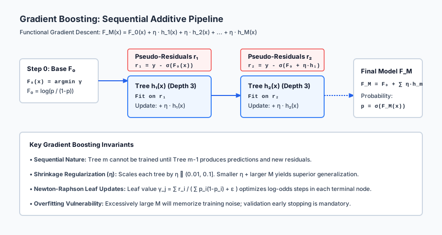
The diagram illustrates how each sequential tree fits the negative gradient before applying shrinkage eta.
Below is the functional gradient descent optimization trajectory:
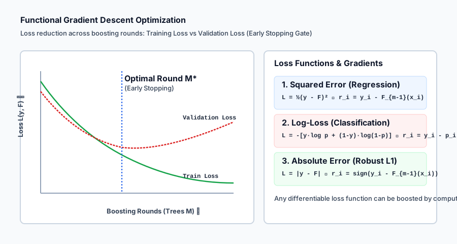
Let us examine real Python code training a Gradient Boosting Classifier and evaluating early stopping:
import numpy as np
from sklearn.datasets import load_breast_cancer
from sklearn.ensemble import GradientBoostingClassifier
from sklearn.model_selection import train_test_split
from sklearn.metrics import accuracy_score, log_loss

# 1. Load Data
cancer = load_breast_cancer()
X, y = cancer.data, cancer.target

X_train, X_test, y_train, y_test = train_test_split(
    X, y, test_size=0.25, stratify=y, random_state=42
)

# 2. Fit Gradient Boosting with Validation Monitoring
gb = GradientBoostingClassifier(
    n_estimators=100,
    learning_rate=0.08,
    max_depth=3,
    subsample=0.85, # Stochastic Gradient Boosting (85% rows)
    validation_fraction=0.20,
    n_iter_no_change=10, # Early stopping patience: 10 rounds
    random_state=42
)
gb.fit(X_train, y_train)

# 3. Evaluate Predictions
test_preds = gb.predict(X_test)
test_probs = gb.predict_proba(X_test)[:, 1]

print("=== Gradient Boosting Clinical Benchmark ===")
print(f"Optimal Trees Trained:    {gb.n_estimators_} (Stopped early from 100)")
print(f"Independent Test Accuracy: {accuracy_score(y_test, test_preds) * 100:.2f}%")
print(f"Test Log-Loss (Deviance): {log_loss(y_test, test_probs):.4f}")

# 4. Inspect Feature Importances
importances = gb.feature_importances_
top_idx = np.argsort(importances)[::-1][:5]
print("\nTop 5 Most Influential Features:")
for idx in top_idx:
    print(f"• {cancer.feature_names[idx]:25s}: {importances[idx]:.4f}")
Implications: security, privacy, performance, scalability, and cost
| Dimension | Characteristic | Practical Implication |
|---|---|---|
| Sequential Compute Bottleneck | Cannot parallelize outer loop across trees. | Training 1,000 trees requires 1,000 sequential passes. Highly optimized histogram algorithms (XGBoost/LightGBM) parallelize the inner split evaluation instead. |
| Inference Latency | O(M * depth). | Evaluating 100 shallow trees takes < 1 ms, making Gradient Boosting suitable for real-time production inference. |
| Differential Privacy Risks | Residuals expose ground truth labels. | In distributed or federated learning, sharing raw gradient residuals r_i = y_i - p_i allows attackers to reconstruct training labels. Gradient clipping and DP noise are required. |
| Hyperparameter Sensitivity | High interaction between eta, M, and max_depth. | Requires systematic tuning (Grid/Random Search or Optuna) compared to Random Forests. |
Alternatives: free, open source, and commercial
| Tool / Framework | Innovation | License / Cost | Best Used For |
|---|---|---|---|
scikit-learn (GradientBoostingClassifier) | Reference Python/C implementation | Free, BSD Open Source | Baseline education, prototyping, small-to-medium tabular datasets. |
HistGradientBoostingClassifier | Histogram binning (inspired by LightGBM) | Free, BSD Open Source | 10x faster training on large datasets directly within scikit-learn. |
XGBoost | Exact second-order Taylor approximation + sparsity | Free, Apache 2.0 | High-performance competitive tabular modeling (Day 165). |
LightGBM | GOSS + Exclusive Feature Bundling | Free, MIT | Ultra-fast training on million-row tabular datasets (Day 165). |
CatBoost | Symmetric oblivious trees + categorical handling | Free, Apache 2.0 | State-of-the-art accuracy on heavy categorical datasets (Day 165). |
Comparison with related concepts
| Characteristic | Random Forests | Gradient Boosting | Deep Neural Networks |
|---|---|---|---|
| Ensemble Logic | Independent parallel trees | Sequential residual correction | Layered differentiable tensor operations |
| Base Learner | Deep, unpruned trees | Shallow, weak trees (depth 3–6) | Neurons with activation functions |
| Overfitting Behavior | Safe: adding trees lowers variance | Vulnerable: adding too many trees overfits | Vulnerable: requires dropout / weight decay |
| Tabular Data Performance | High | State-of-the-Art | Often requires extensive tuning on tabular data |
| Feature Scaling | Not required | Not required | Strictly required |
When to use it — and when not to
When to USE Gradient Boosting:
- When Maximum Predictive Accuracy on Tabular Data is Required: The unmatched champion on structured business datasets.
- Custom Loss Functions and Objectives: When your business problem penalizes false positives 10x more than false negatives.
- Non-Linear Data with Complex Interactions: Easily captures multi-feature conditionals without manual feature crosses.
When NOT to use Gradient Boosting:
- Unstructured Data (Images, Audio, Natural Language): Convolutional Networks and Transformers vastly outperform trees on spatial and sequential data.
- Need for Embarrassingly Parallel Fast Training: When you have a 128-core server and want to train 1,000 independent trees in 2 seconds (use Random Forest).
- Zero Hyperparameter Tuning Budget: If you cannot tune
learning_rateor set up early stopping, a Random Forest is safer out of the box.
Knowledge check
- Additive Model Form:
F_M(x) = F_0(x) + sum eta * h_m(x). - Pseudo-Residual: Negative loss gradient
r_im = - [ dL / dF ]. - Log-Loss Negative Gradient:
r_i = y_i - sigmoid(F(x_i)). - Newton-Raphson Leaf Update:
gamma_j = sum(r) / sum(p * (1 - p)).
Hands-on exercise
In this hands-on exercise, you will implement pseudo-residual calculation for classification, fit a 3-iteration boosting loop on a 1D dataset, and observe residual convergence.
import numpy as np
from sklearn.tree import DecisionTreeRegressor

# Step 1: Binary Classification Dataset
X = np.array([[1.0], [2.0], [3.0], [4.0], [5.0], [6.0]])
y = np.array([0, 0, 0, 1, 1, 1])

def sigmoid(z):
    return 1.0 / (1.0 + np.exp(-np.clip(z, -30.0, 30.0)))

# Step 2: Initialize F0 (Log-Odds)
p_mean = np.mean(y) # 0.50
F0 = np.log(p_mean / (1.0 - p_mean)) # 0.0
F = np.full(len(y), F0)

print(f"Step 0: Initial F0 = {F0:.2f}, Initial Probabilities = {sigmoid(F)}")

# Step 3: Run 3 Boosting Iterations
learning_rate = 0.5
trees = []

for m in range(1, 4):
    p = sigmoid(F)
    residuals = y - p

    # Fit shallow regression stump to residuals
    stump = DecisionTreeRegressor(max_depth=1, random_state=42)
    stump.fit(X, residuals)

    # Update additive model
    update = stump.predict(X)
    F += learning_rate * update
    trees.append(stump)

    print(f"\nIteration {m}:")
    print(f"  Pseudo-Residuals: {np.round(residuals, 3)}")
    print(f"  Updated Probabilities: {np.round(sigmoid(F), 3)}")

print("\nFinal Predicted Classes:", (sigmoid(F) >= 0.5).astype(int))
Expected output
Step 0: Initial F0 = 0.00, Initial Probabilities = [0.5 0.5 0.5 0.5 0.5 0.5]

Iteration 1:
  Pseudo-Residuals: [-0.5 -0.5 -0.5  0.5  0.5  0.5]
  Updated Probabilities: [0.378 0.378 0.378 0.622 0.622 0.622]

Iteration 2:
  Pseudo-Residuals: [-0.378 -0.378 -0.378  0.378  0.378  0.378]
  Updated Probabilities: [0.291 0.291 0.291 0.709 0.709 0.709]

Iteration 3:
  Pseudo-Residuals: [-0.291 -0.291 -0.291  0.291  0.291  0.291]
  Updated Probabilities: [0.231 0.231 0.231 0.769 0.769 0.769]

Final Predicted Classes: [0 0 0 1 1 1]
Validate your work
- Verify that
residualsdecrease in absolute magnitude with each iteration. - Confirm that predicted probabilities move towards
0.0for class 0 and1.0for class 1. - Train
GradientBoostingClassifier(n_estimators=30, learning_rate=0.1)on breast cancer and verify accuracy>= 95%.
Troubleshooting
- Predictions Exploding to Inf: Clip the raw score
Fto[-30, 30]before computingsigmoid(F). - Zero Loss Reduction: Ensure
learning_rate > 0.0and that base trees havemax_depth >= 1.
Common mistakes
- Using Deep Trees (
max_depth > 8): In boosting, deep trees overfit the residuals immediately; stick tomax_depth = 3to6. - Forgetting Early Stopping: Always monitor a validation set and stop adding trees when validation loss stalls.
Practice assignment
- Implement Huber Loss for Robust Regression:
Derive the pseudo-residual for Huber loss with threshold delta:
r_i = y_i - F(x_i)if|y_i - F| <= delta, elsedelta * sign(y_i - F(x_i)). Build a custom Gradient Boosting Regressor using Huber loss and test on a dataset with synthetic outliers. - Implement Subsample (Stochastic Gradient Boosting):
Add a
subsample = 0.8parameter toGradientBoostingClassifierScratchthat randomly samples 80% of rows at each iteration before computing residuals.
Extension challenge
Implement Exact Second-Order (Newton) Tree Boosting (XGBoost Engine from Scratch):
- Instead of fitting a standard CART tree to first derivatives, implement a split criterion that directly uses both first derivatives
g_iand second derivativesh_i:Gain = 0.5 * [ (G_L^2 / (H_L + lambda)) + (G_R^2 / (H_R + lambda)) - (G^2 / (H + lambda)) ] - gamma - Benchmark your custom second-order boosting engine against scikit-learn’s
GradientBoostingClassifier.
Quiz
Q1. What is the fundamental difference in training strategy between Bagging (Random Forests) and Boosting (Gradient Boosting)?
- Bagging trains independent trees in parallel on bootstrap samples to reduce variance; Boosting trains shallow trees sequentially to fit the residual errors of prior trees to reduce bias and variance
- Bagging uses gradient descent; Boosting uses random guessing
- Bagging is for classification only; Boosting is for regression only
- Bagging requires normalized features; Boosting does not
Show answer
Answer: A. Bagging trains independent trees in parallel on bootstrap samples to reduce variance; Boosting trains shallow trees sequentially to fit the residual errors of prior trees to reduce bias and variance
Random Forests train diverse trees independently in parallel to lower variance. Gradient Boosting builds trees sequentially, with each new tree taking a step in function space along the negative gradient of the loss.
Q2. What is a "pseudo-residual" in Gradient Boosting?
- The negative gradient of the loss function with respect to current model predictions: r_im = - [ d L(y_i, F(x_i)) / d F(x_i) ]
- A random number used for regularization
- The difference between feature values and their mean
- The out-of-bag classification error
Show answer
Answer: A. The negative gradient of the loss function with respect to current model predictions: r_im = - [ d L(y_i, F(x_i)) / d F(x_i) ]
Gradient boosting performs gradient descent in function space. The negative gradient points in the direction of steepest descent, which acts as the target signal (pseudo-residual) for the next tree.
Q3. For Binary Cross-Entropy loss L(y, F), what is the pseudo-residual r_i where p_i = sigmoid(F(x_i))?
- r_i = y_i - p_i
- r_i = y_i * log(p_i)
- r_i = (y_i - p_i)^2
- r_i = 1 / (1 + exp(-F_i))
Show answer
Answer: A. r_i = y_i - p_i
Differentiating binary cross-entropy with respect to the raw log-odds score F yields the negative gradient r_i = y_i - p_i.
Q4. Why is shrinkage (learning rate eta in (0, 1]) essential in Gradient Boosting?
- It scales down the contribution of each new tree, forcing the model to learn slowly across many trees and preventing rapid overfitting to training noise
- It speeds up tree training time
- It reduces the memory size of the tree
- It converts regression trees into classification trees
Show answer
Answer: A. It scales down the contribution of each new tree, forcing the model to learn slowly across many trees and preventing rapid overfitting to training noise
Shrinkage acts as a powerful regularizer. Taking small steps along the gradient (e.g. eta = 0.05) leaves room for future trees to correct errors on diverse sub-patterns rather than memorizing early training residuals.
Q5. What is the initial constant prediction F_0 for binary classification in Gradient Boosting?
- The log-odds of the positive class: F_0 = log(p / (1 - p)) where p is the proportion of y=1 in the training set
- 0.0 for all datasets
- The mean target value p
- A randomly initialized weight matrix
Show answer
Answer: A. The log-odds of the positive class: F_0 = log(p / (1 - p)) where p is the proportion of y=1 in the training set
Setting F_0 to the empirical log-odds minimizes initial binary cross-entropy loss before any trees are added.
Q6. Why do Gradient Boosted Trees use shallow decision trees (depth 3 to 6) as base learners, while Random Forests use deep unpruned trees?
- Boosting sequentially reduces bias by adding trees; using shallow base learners (weak learners) prevents individual trees from overfitting while the additive ensemble builds capacity
- Shallow trees cannot compute gradients
- Deep trees cannot be trained with shrinkage
- Shallow trees are required for GPU execution
Show answer
Answer: A. Boosting sequentially reduces bias by adding trees; using shallow base learners (weak learners) prevents individual trees from overfitting while the additive ensemble builds capacity
Random Forests average deep, low-bias trees to reduce variance. Boosting uses shallow, high-bias trees and sequentially drives both bias and variance down through additive gradient steps.
Q7. What happens if you train Gradient Boosting for 5,000 trees with learning rate eta = 0.3 without early stopping?
- The model will severely overfit the training set, driving training loss to zero while test error increases
- The model will asymptotically converge to the optimal Bayes error without overfitting
- The trees will automatically collapse to depth 1
- The learning rate will automatically decay to zero
Show answer
Answer: A. The model will severely overfit the training set, driving training loss to zero while test error increases
Unlike Random Forests, Gradient Boosting CAN overfit if too many trees are added. Monitoring validation loss with early stopping is mandatory in production.
Q8. What is the purpose of Newton-Raphson leaf value adjustment in classification trees?
- Because standard regression tree leaves output simple average residuals, Newton-Raphson divides by the second derivative (curvature) to find the optimal step size in log-odds space: sum(r) / sum(p*(1-p))
- To sort the feature thresholds
- To convert probabilities to integers
- To calculate Out-of-Bag error
Show answer
Answer: A. Because standard regression tree leaves output simple average residuals, Newton-Raphson divides by the second derivative (curvature) to find the optimal step size in log-odds space: sum(r) / sum(p*(1-p))
Since log-loss is non-linear, a single second-order Newton-Raphson step gamma = -g / H = sum(r) / sum(p*(1-p)) computes the exact optimal leaf weight update.
Glossary
- Gradient Boosting
- An ensemble method that builds an additive model sequentially by training base estimators (typically shallow decision trees) on the negative gradient of a differentiable loss function.
- Functional Gradient Descent
- The optimization paradigm of taking gradient steps in the infinite-dimensional space of functions, rather than optimizing a fixed parameter vector in Euclidean space.
- Pseudo-Residual
- The negative gradient of the loss function with respect to model predictions (-dL/dF), serving as the training target for each subsequent boosting iteration.
- Shrinkage (Learning Rate)
- A regularization scaling factor eta in (0, 1] that multiplies the output of each newly added tree, controlling the step size along the functional gradient.
- Additive Model
- A model structure of the form F(x) = sum(eta * h_m(x)), where the final prediction is a linear combination of base learners.
- Newton-Raphson Step
- A second-order optimization update that divides the first derivative (gradient) by the second derivative (Hessian) to optimize leaf values for non-quadratic loss functions.
- Weak Learner
- A base model (such as a depth-3 decision tree stump) that performs only slightly better than random guessing on its own, but combines into a strong learner when boosted.
- Stochastic Gradient Boosting
- An extension where a random subsample of training instances (and/or features) is drawn without replacement at each iteration to compute pseudo-residuals.
- Early Stopping
- Halting the boosting iterations when performance on a held-out validation dataset stops improving for a specified number of rounds (patience).
- Deviance
- Twice the negative log-likelihood (log-loss), commonly used as the loss metric for binary classification gradient boosting.
Sources and further reading
- Greedy Function Approximation: A Gradient Boosting Machine — The Annals of Statistics (Jerome H. Friedman) (accessed 2026-08-29)
- Stochastic Gradient Boosting — Computational Statistics & Data Analysis (Jerome H. Friedman) (accessed 2026-08-29)
- The Elements of Statistical Learning (Chapter 10: Boosting and Additive Trees) — Springer (Hastie, Tibshirani, Friedman) (accessed 2026-08-29)
Kept in this browser, no account needed. Your progress page turns the whole record into one link you can bookmark or open on another device.