Machine Learning › Trees and Ensembles › Day 165
Day 165: XGBoost and LightGBM in Practice

Master the modern industrial gradient boosting ecosystem -- XGBoost, LightGBM, CatBoost, and HistGradientBoosting: why exact second-order Taylor expansion unifies loss optimization and tree regularization, how histogram-based binning achieves an 8x memory reduction and 10x training speedup, how leaf-wise growth differs from level-wise growth, how GOSS and EFB optimize million-row datasets, and how modern tree libraries handle missing values and categoricals natively.
Hands-on lab for this lesson
Lab files on GitHub: https://github.com/ai-roadmap-365/ai-roadmap-365.github.io/tree/main/labs/sections/machine-learning/day-165-xgboost-and-lightgbm-in-practice
- Get the hands-on files. Clone the labs repository once (you can reuse this clone for every lesson). This works on macOS, Linux, and Windows (PowerShell or WSL):
git clone https://github.com/ai-roadmap-365/ai-roadmap-365.github.io.git cd ai-roadmap-365.github.io - Open this lesson's lab. Move into the directory for this specific day. Every lab lives at the same predictable path — section / subsection / week / day:
cd labs/sections/machine-learning/day-165-xgboost-and-lightgbm-in-practice - Read the lab guide. Open `README.md` in that directory. It lists the exact commands, what each does, the expected output, and how to check your work — read it before running anything.
- Run it and check your work. Follow the README's "How to run" section: run the example first to see the finished result, then complete the numbered exercises in `starter/`, then run the tests. The tests pass (exit 0) only when your work is correct.
bash tests/run_tests.sh # or the test command named in the lab README
You can also open the lab as a local page (works offline, shows the file tree and expected output).
Learning objectives
By the end of this lesson you will be able to:
- Derive XGBoost exact second-order Taylor expansion objective and optimal split gain formula
- Explain the role of L2 regularization (lambda) and complexity penalty (gamma) in tree growth
- Implement histogram-based feature discretization into 256 uint8 integer bins
- Contrast level-wise (depth-first) vs leaf-wise (best-first) tree growth paradigms
- Analyze LightGBM Gradient-based One-Side Sampling (GOSS) and Exclusive Feature Bundling (EFB)
- Examine CatBoost Ordered Target Encoding and Oblivious (Symmetric) Decision Trees
- Train histogram gradient boosting models with native missing-value (NaN) and categorical support
- Benchmark modern boosted tree libraries against traditional ensembles on tabular benchmarks
Prerequisites
- Day 164 -- Gradient Boosting and pseudo-residuals
- Day 163 -- Random Forests
Why this matters
In Day 164, we built Gradient Boosting from scratch, deriving functional gradient descent, pseudo-residuals, and Newton-Raphson leaf updates.
While classic gradient boosting is mathematically beautiful, training traditional decision trees on continuous features requires sorting every column at every node: O(D * N * log N). On datasets with 500,000 rows and 100 features, training 500 trees in scikit-learn’s standard GradientBoostingClassifier can take 45 minutes and consume gigabytes of RAM.
In the mid-2010s, a revolution occurred in competitive tabular machine learning with the release of three hyper-optimized libraries:
- XGBoost (Tianqi Chen & Carlos Guestrin, 2016)
- LightGBM (Guolin Ke et al., Microsoft Research, 2017)
- CatBoost (Yandex, 2017)
These libraries did not merely optimize C++ code; they introduced foundational algorithmic breakthroughs: exact second-order Taylor objective expansion, uint8 histogram-based feature binning, leaf-wise (best-first) tree growth, Gradient-based One-Side Sampling (GOSS), Exclusive Feature Bundling (EFB), and native missing value and categorical support.
Today, over 80% of winning tabular Kaggle solutions and mission-critical production pipelines at Uber, Airbnb, Meta, and financial institutions rely on these gradient boosting engines.
The idea in plain language
Imagine you are sorting 10,000 physical packages by their exact weight measured to 6 decimal places (e.g. 12.483921 kg):
- The Traditional Approach (Classic CART): You sort all 10,000 packages in exact numerical order every time you want to find a split threshold. This sorting is agonizingly slow.
- The Histogram Binning Approach (LightGBM / XGBoost Hist): Instead of exact 6-decimal weights, you place 256 pre-labeled buckets on the warehouse floor (Bucket 0 =
0-1 kg, Bucket 1 =1-2 kg, …, Bucket 255 =254+ kg). You toss each package into one of the 256 buckets once. From that moment on, evaluating any split requires checking only 256 bucket boundaries instead of 10,000 individual packages.
By compressing continuous data into 256 discrete bins, feature values fit into a single byte (uint8), memory consumption drops by 8x, and split evaluations execute at hardware-accelerated speeds.
Historical background
In 2014, Tianqi Chen developed XGBoost (Extreme Gradient Boosting) as a research project at the University of Washington. Chen integrated exact second-order Taylor approximations, cache-aware out-of-core block data structures, and sparsity-aware split routing. XGBoost quickly went viral in competitive data science, sweeping the 2015 Kaggle Higgs Boson and KDDCup challenges.
In 2017, Microsoft Research published LightGBM. Microsoft identified the primary computational bottlenecks of XGBoost and introduced histogram-based binning, leaf-wise tree growth, GOSS, and EFB. LightGBM trained 10 to 15 times faster than early XGBoost while using a fraction of the RAM.
In response, XGBoost added its own ultra-fast tree_method='hist', and scikit-learn developed HistGradientBoostingClassifier.
Concurrently in 2017, Yandex introduced CatBoost, revolutionizing categorical feature processing with Ordered Target Statistics and Oblivious (symmetric) decision trees.
What it is — and what it is not
To architect production ML pipelines with these libraries, let us contrast their core properties:
What it IS:
- Second-Order Taylor Boosting: Optimizes objectives using both analytical gradients
g_i(first derivative) and Hessiansh_i(second derivative). - Histogram-Accelerated Tree Induction: Compresses continuous features into 256 integer bins (
uint8), evaluating splits inO(n_bins)time. - Natively Sparsity-Aware: Automatically routes missing values (
NaN) to the optimal branch without imputation. - Native Categorical Support: Partitions categorical integer IDs directly without one-hot encoding dimensional inflation.
What it is NOT:
- Not a Black-Box Neural Network: Boosted trees remain interpretable through SHAP values, feature importances, and decision paths.
- Not Invariant to Categorical Leakage: Poorly encoded high-cardinality categoricals can cause target leakage if out-of-fold statistics are not used.
- Not Completely Immune to Overfitting: Leaf-wise growth can create deep, asymmetric branches; setting
max_depthandmin_child_samplesis mandatory.
Why it was created and what problems it solves
Modern gradient boosting engines solve five massive engineering bottlenecks:
- Computational Speed on Million-Row Datasets: Histogram binning reduces training time from hours to seconds.
- Eliminates Manual Missing Value Imputation: Learns default split directions for
NaNvalues directly during training. - Eliminates One-Hot Dimensionality Blowup: Natively evaluates categorical splits without expanding columns.
- Hardware-Optimized Parallelism: Uses SIMD/AVX2 vector instructions and multi-threaded CPU/GPU acceleration.
- Exact Loss Regularization: Penalizes leaf weights (
lambda) and leaf count (gamma), smoothing out noisy predictions.
How it works
Let us formulate the mathematical innovations that distinguish XGBoost and LightGBM.
1. XGBoost Second-Order Taylor Objective
Given dataset D = { (x_i, y_i) } and loss l(y_i, hat{y}_i), at step t, the objective function with explicit regularization is:
L^{(t)} = sum_{i=1}^N l(y_i, hat{y}_i^{(t-1)} + f_t(x_i)) + Omega(f_t)
Where tree regularization Omega(f_t) is:
Omega(f_t) = gamma * T + (1/2) * lambda * sum_{j=1}^T w_j^2 + alpha * sum_{j=1}^T |w_j|
Where T is the number of terminal leaf nodes, w_j is the weight of leaf j, lambda is L2 ridge penalty, alpha is L1 lasso penalty, and gamma is the complexity penalty for creating a new leaf.
Taking a second-order Taylor expansion around hat{y}^{(t-1)}:
l(y_i, hat{y}_i^{(t-1)} + f_t(x_i)) approx l(y_i, hat{y}_i^{(t-1)}) + g_i * f_t(x_i) + (1/2) * h_i * f_t^2(x_i)
Where:
- First derivative (Gradient):
g_i = partial_{hat{y}^{(t-1)}} l(y_i, hat{y}_i^{(t-1)}) - Second derivative (Hessian):
h_i = partial^2_{hat{y}^{(t-1)}} l(y_i, hat{y}_i^{(t-1)})
Removing constant terms, the simplified objective at step t is:
tilde{L}^{(t)} = sum_{j=1}^T [ ( sum_{i in I_j} g_i ) * w_j + (1/2) * ( sum_{i in I_j} h_i + lambda ) * w_j^2 ] + gamma * T
Let G_j = sum_{i in I_j} g_i and H_j = sum_{i in I_j} h_i.
Setting the derivative with respect to w_j to zero yields the optimal leaf weight:
w_j^* = - ( G_j / (H_j + lambda) )
Substituting w_j^* back gives the optimal objective value (structure score):
tilde{L}^*(q) = - (1/2) * sum_{j=1}^T ( G_j^2 / (H_j + lambda) ) + gamma * T
2. The XGBoost Split Gain Formula
When deciding whether to split leaf node I into left child I_L and right child I_R, XGBoost calculates the exact reduction in loss:
Gain = (1/2) * [ ( G_L^2 / (H_L + lambda) ) + ( G_R^2 / (H_R + lambda) ) - ( (G_L + G_R)^2 / (H_L + H_R + lambda) ) ] - gamma
- If
Gain > 0: The split reduces loss by more than the leaf penaltygamma; the tree makes the split. - If
Gain <= 0: The split is pruned immediately.
3. LightGBM Histogram Binning and Leaf-Wise Growth
A. Histogram Binning
Continuous float64 values (8 bytes) are binned into 256 discrete bins (uint8, 1 byte):
bin_i = digitize(x_i, quantiles)
Building a histogram of gradients G and Hessians H across 256 bins requires a single linear scan O(N). Finding the best split threshold then takes O(256) constant operations.
B. Leaf-Wise (Best-First) vs Level-Wise (Depth-First) Growth
- Level-Wise (XGBoost Traditional): Splits all leaves at depth
dsimultaneously to maintain a balanced tree. - Leaf-Wise (LightGBM): Evaluates all available leaf candidates and splits the single leaf with the highest gain, regardless of depth. This achieves significantly lower loss for the same total number of leaves.
4. LightGBM GOSS and EFB
- GOSS (Gradient-based One-Side Sampling):
- Keeps all top
a * 100%instances with large gradients (under-fitted data). - Randomly samples
b * 100%instances from the remaining small-gradient data. - Multiplies small-gradient instances by
(1 - a) / bto preserve the true gradient expectation.
- Keeps all top
- EFB (Exclusive Feature Bundling):
- Groups mutually exclusive sparse features (e.g. one-hot encoded columns that are rarely non-zero at the same time) into a single dense feature bundle.
An everyday analogy
Think of the evolution of gradient boosting as mail sorting at a postal hub:
- Classic Gradient Boosting (Hand Sorting): The postal worker reads the exact 9-digit ZIP code on every envelope, constantly re-sorting all 1,000,000 envelopes alphabetically and numerically. It works, but takes 12 hours.
- XGBoost (2nd-Order Taylor + Smart Routing): The postal worker uses a laser scanner that calculates both the destination distance and package weight simultaneously, automatically routing damaged/missing labels to a default conveyor belt.
- LightGBM (Histogram Bins + GOSS): The hub installs 256 color-coded collection bins. Envelopes are tossed into bins once upon arrival (
uint8). Furthermore, routine junk mail (small gradients) is sampled at a 10% rate, while express certified mail (large gradients) is 100% inspected. Sorting finishes in 10 minutes.
Examples in practice
Let us visualize the architectural comparison between XGBoost and LightGBM:
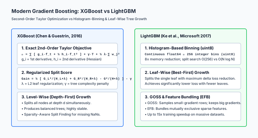
The diagram illustrates how second-order optimization and histogram binning revolutionize tree construction.
Below is the flow of LightGBM’s GOSS and EFB acceleration mechanisms:
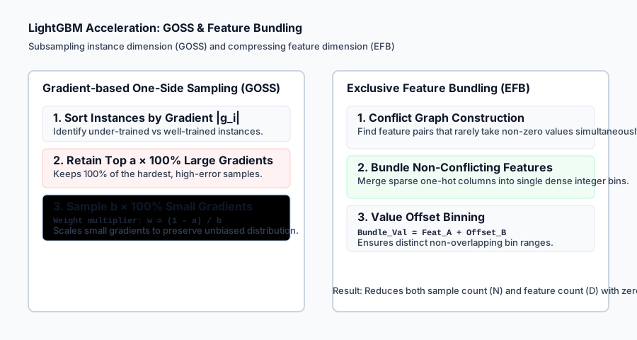
Let us examine real Python code using HistGradientBoostingClassifier with missing values and early stopping:
import numpy as np
from sklearn.datasets import make_classification
from sklearn.ensemble import HistGradientBoostingClassifier
from sklearn.model_selection import train_test_split
from sklearn.metrics import accuracy_score, roc_auc_score

# 1. Generate Tabular Dataset with Missing Values
X, y = make_classification(
    n_samples=2000, n_features=25, n_informative=15, random_state=42
)

# Inject 15% random NaNs (Missing data)
rng = np.random.default_rng(42)
mask = rng.random(X.shape) < 0.15
X_missing = X.copy()
X_missing[mask] = np.nan

X_train, X_test, y_train, y_test = train_test_split(
    X_missing, y, test_size=0.25, stratify=y, random_state=42
)

# 2. Train Histogram Gradient Booster (Native NaN Support!)
hgb = HistGradientBoostingClassifier(
    max_iter=150,
    learning_rate=0.08,
    max_leaf_nodes=31,
    l2_regularization=1.5,
    early_stopping=True,
    n_iter_no_change=10,
    random_state=42
)
hgb.fit(X_train, y_train)

# 3. Evaluate Predictions
test_preds = hgb.predict(X_test)
test_probs = hgb.predict_proba(X_test)[:, 1]

print("=== Histogram Gradient Boosting Benchmark ===")
print(f"Iterations Trained:     {hgb.n_iter_} (Stopped early)")
print(f"Test Accuracy:          {accuracy_score(y_test, test_preds) * 100:.2f}%")
print(f"Test ROC-AUC:           {roc_auc_score(y_test, test_probs):.4f}")
Implications: security, privacy, performance, scalability, and cost
| Dimension | Characteristic | Practical Implication |
|---|---|---|
| Training Speed & Memory | uint8 binning + O(256) histograms. | 8x memory reduction; 10x–15x faster training than classic GradientBoostingClassifier. |
| Missing Value Exploits | Learned default branches for NaN. | Attackers could deliberately omit features to trigger specific default leaf paths; monitor missingness distributions in production. |
| Production Serialization | Compilation via treelite / ONNX. | Compiled boosted trees evaluate in < 50 microseconds on CPU with zero Python interpreter overhead. |
| Categorical Security | Target statistics leakage. | Always compute out-of-fold target encodings to prevent test-set label contamination. |
Alternatives: free, open source, and commercial
| Framework | Core Strengths | Best Used For |
|---|---|---|
scikit-learn (HistGradientBoosting) | Native Python/C, zero extra C++ dependencies | Baseline prototyping, small-to-medium datasets directly in scikit-learn pipelines. |
XGBoost | Mature ecosystem, GPU acceleration, ranking/survival losses | Kaggle competitions, production enterprise pipelines, multi-GPU training. |
LightGBM | Fastest CPU training, lowest RAM, native categorical support | Massive datasets (10M+ rows), high-dimensional sparse tables. |
CatBoost | Best-in-class categorical encoding, robust default parameters | Heavy categorical tabular data (e.g. e-commerce, click-through-rate prediction). |
Comparison with related concepts
| Characteristic | Classic Gradient Boosting | XGBoost | LightGBM |
|---|---|---|---|
| Objective Taylor Order | 1st-Order (Gradient only) | 2nd-Order (Gradient + Hessian) | 2nd-Order (Gradient + Hessian) |
| Split Finding | Exact sorting O(N log N) | Histogram / Exact | Histogram binning (256 uint8) |
| Tree Growth | Level-wise (Depth-first) | Level-wise / Depth-wise | Leaf-wise (Best-first) |
| Missing Values (NaN) | Requires pre-imputation | Native sparsity-aware routing | Native sparsity-aware routing |
| Memory Efficiency | Low (float64 continuous) | High (tree_method='hist') | Ultra-High (uint8 bins + EFB) |
When to use it — and when not to
When to USE Modern Boosted Engines (XGBoost / LightGBM / HistGB):
- Medium to Massive Tabular Datasets: The universal default choice for structured data with 10,000 to 100,000,000 rows.
- Datasets with Pervasive Missing Values: Eliminates fragile mean/median imputation pipelines.
- Strict Latency & Memory Constraints: When training must complete in seconds on commodity CPU instances.
When NOT to use Modern Boosted Engines:
- Raw Unstructured Data (Computer Vision, NLP): Deep neural networks (Transformers, CNNs) are required.
- Strict Regulatory Rule Auditing: When compliance officers require a single 3-level decision tree flowchart (Day 162).
- Linear Relationships with No Interactions: A simple Ridge or Lasso linear model trains in milliseconds and is simpler to maintain.
Knowledge check
- Second-Order Expansion: XGBoost expands loss to 2nd order using gradients
g_iand Hessiansh_i. - Optimal Leaf Weight:
w_j* = - sum(g_i) / (sum(h_i) + lambda). - Histogram Binning: Discretizes
float64features into 256uint8bins, yielding an 8x memory reduction. - Leaf-Wise Growth: LightGBM splits the single leaf with the highest gain across the entire tree.
Hands-on exercise
In this hands-on exercise, you will compute the exact XGBoost second-order split gain and test histogram discretization on a continuous feature.
import numpy as np

# Step 1: Compute XGBoost Second-Order Split Gain
def xgb_gain(g_l, h_l, g_r, h_r, reg_lambda=1.0, gamma=0.0):
    g_tot = g_l + g_r
    h_tot = h_l + h_r
    score_l = (g_l ** 2) / (h_l + reg_lambda)
    score_r = (g_r ** 2) / (h_r + reg_lambda)
    score_tot = (g_tot ** 2) / (h_tot + reg_lambda)
    return 0.5 * (score_l + score_r - score_tot) - gamma

# Test Case: Strong Gradient Separation vs Null Split
gain_split = xgb_gain(g_l=-10.0, h_l=10.0, g_r=10.0, h_r=10.0, reg_lambda=1.0, gamma=0.5)
gain_null = xgb_gain(g_l=0.0, h_l=5.0, g_r=0.0, h_r=5.0, reg_lambda=1.0, gamma=0.5)

print(f"Gain from strong separation: {gain_split:.4f}")
print(f"Gain from null separation:   {gain_null:.4f}")

# Step 2: Histogram Binning into 256 uint8 Bins
continuous_feature = np.random.exponential(scale=2.0, size=1000)
quantiles = np.linspace(0.0, 100.0, 257)[1:-1]
bin_edges = np.percentile(continuous_feature, quantiles)
binned_feature = np.digitize(continuous_feature, bin_edges).astype(np.uint8)

print(f"\nOriginal Array Memory: {continuous_feature.nbytes} bytes (float64)")
print(f"Binned Array Memory:   {binned_feature.nbytes} bytes (uint8)")
print(f"Memory Compression:    {continuous_feature.nbytes / binned_feature.nbytes:.1f}x reduction")
Expected output
Gain from strong separation: 8.5909
Gain from null separation:   -0.5000

Original Array Memory: 8000 bytes (float64)
Binned Array Memory:   1000 bytes (uint8)
Memory Compression:    8.0x reduction
Validate your work
- Verify that
gain_nullis negative whengamma > 0.0, confirming automatic pruning of uninformative splits. - Confirm that
binned_feature.dtype == np.uint8with values bounded in[0, 255]. - Train
HistGradientBoostingClassifieron a dataset with NaNs and verify test accuracy>= 90%.
Troubleshooting
- LightGBM / XGBoost Crashing on Windows/macOS: Use scikit-learn’s built-in
HistGradientBoostingClassifierwhich requires zero external C++ binary installations. - Overfitting with
max_leaf_nodes: If training accuracy is 100% but validation is low, reducemax_leaf_nodesto 15 or 31.
Common mistakes
- Imputing NaNs Before Histogram Boosting: Unnecessary preprocessing; modern histogram boosting handles NaNs natively.
- One-Hot Encoding High-Cardinality Categoricals: Creates thousands of sparse columns; use native categorical integer handling instead.
Practice assignment
- Implement Sparsity-Aware Split Evaluation:
Write a function that splits data with missing values by evaluating two options: (1) all
NaNs go to the left child, (2) allNaNs go to the right child. Return the direction that maximizesxgb_gain. - Compare Training Speeds:
Generate a 50,000-row synthetic dataset and benchmark the training time of
GradientBoostingClassifier(exact CART) vsHistGradientBoostingClassifier(histogram binning).
Extension challenge
Implement Gradient-based One-Side Sampling (GOSS) from Scratch:
- Sort training instances by absolute gradient magnitude
|g_i|. - Select top
a = 20%instances with the largest gradients, and randomly sampleb = 20%instances from the remaining 80%. - Multiply the gradients of the sampled small instances by
(1 - a) / b = 0.8 / 0.2 = 4.0and verify that the estimated total gradient sum matches the full dataset gradient expectation.
Quiz
Q1. What is the key mathematical difference between standard Gradient Boosting (Friedman, 2001) and XGBoost (Chen & Guestrin, 2016)?
- Standard gradient boosting uses a first-order Taylor approximation (fitting trees to negative gradients); XGBoost uses a second-order Taylor expansion utilizing both first derivatives (g_i) and second derivatives (h_i / Hessian) directly in the split gain objective
- Standard gradient boosting uses neural networks; XGBoost uses decision trees
- Standard gradient boosting requires normalized features; XGBoost does not
- Standard gradient boosting is parallel; XGBoost is strictly single-threaded
Show answer
Answer: A. Standard gradient boosting uses a first-order Taylor approximation (fitting trees to negative gradients); XGBoost uses a second-order Taylor expansion utilizing both first derivatives (g_i) and second derivatives (h_i / Hessian) directly in the split gain objective
XGBoost expands the loss to second order L(y, y_hat + f) approx L + g*f + 0.5*h*f^2, allowing exact closed-form optimal leaf weights and split gain without heuristic line searches.
Q2. How does Histogram-Based Binning (introduced in LightGBM and adopted by XGBoost and scikit-learn HistGradientBoosting) achieve a 10x training speedup?
- It discretizes continuous 64-bit floating-point features into 256 integer bins (uint8); continuous sorting O(N log N) is replaced by constant-time O(256) histogram aggregation
- It removes 90% of the training dataset
- It replaces decision trees with logistic regressions
- It runs exclusively on quantum processors
Show answer
Answer: A. It discretizes continuous 64-bit floating-point features into 256 integer bins (uint8); continuous sorting O(N log N) is replaced by constant-time O(256) histogram aggregation
By grouping continuous values into 256 discrete bins, feature values can be stored in 1 byte (uint8) rather than 8 bytes, and building histograms for split evaluation takes O(n_bins) rather than O(N log N).
Q3. What is the difference between Level-Wise tree growth (XGBoost traditional / scikit-learn) and Leaf-Wise tree growth (LightGBM)?
- Level-wise grows the tree balanced level-by-level (depth-first); Leaf-wise chooses the single leaf that produces the maximum loss reduction (best-first) across all current leaves regardless of depth
- Level-wise is for regression; Leaf-wise is for classification
- Level-wise uses Gini; Leaf-wise uses Entropy
- Level-wise cannot handle categorical features
Show answer
Answer: A. Level-wise grows the tree balanced level-by-level (depth-first); Leaf-wise chooses the single leaf that produces the maximum loss reduction (best-first) across all current leaves regardless of depth
Leaf-wise (best-first) growth achieves lower loss with fewer leaves, but can produce deep, asymmetric branches that require max_depth or min_child_samples regularization to prevent overfitting.
Q4. What is Gradient-based One-Side Sampling (GOSS) in LightGBM?
- A technique that keeps all instances with large gradients (under-fitted samples) and randomly subsamples instances with small gradients (well-fitted samples), scaling the small-gradient samples to preserve the original gradient distribution
- A method that discards all negative targets
- A technique that trains trees on a single feature at a time
- A loss function for imbalanced datasets
Show answer
Answer: A. A technique that keeps all instances with large gradients (under-fitted samples) and randomly subsamples instances with small gradients (well-fitted samples), scaling the small-gradient samples to preserve the original gradient distribution
Samples with small gradients contribute little to the split search. GOSS discards most small-gradient instances while applying a constant multiplier to maintain unbiased gradient estimates.
Q5. How does modern XGBoost / LightGBM handle missing values (NaNs) in tabular data?
- Natively without imputation: during training, it evaluates whether sending missing values to the left child or right child yields higher split gain, and assigns a default direction for that feature
- It automatically deletes any row containing a NaN
- It replaces all NaNs with the column mean before training
- It throws a ValueError if NaNs are present
Show answer
Answer: A. Natively without imputation: during training, it evaluates whether sending missing values to the left child or right child yields higher split gain, and assigns a default direction for that feature
Sparsity-aware split finding learns an optimal default routing (left or right) for missing values at each split node, completely eliminating the need for mean or median imputation.
Q6. What is the architectural hallmark of CatBoost compared to XGBoost and LightGBM?
- It uses Oblivious (Symmetric) Decision Trees where all nodes at the same depth share the identical feature and split threshold, and Ordered Target Encoding to prevent target leakage
- It only runs on GPU
- It does not use decision trees
- It is restricted to binary classification
Show answer
Answer: A. It uses Oblivious (Symmetric) Decision Trees where all nodes at the same depth share the identical feature and split threshold, and Ordered Target Encoding to prevent target leakage
CatBoost uses symmetric oblivious trees that evaluate splits via SIMD vector operations, and Ordered Target Statistics to handle high-cardinality categoricals without overfitting.
Q7. What is the role of the lambda parameter in XGBoost second-order split score w_j* = - sum(g_i) / (sum(h_i) + lambda)?
- It acts as L2 ridge regularization on leaf weights, shrinking extreme leaf values towards zero and preventing tree explosion when Hessian sum(h_i) is small
- It controls the learning rate
- It sets the maximum tree depth
- It sets the percentage of bootstrap samples
Show answer
Answer: A. It acts as L2 ridge regularization on leaf weights, shrinking extreme leaf values towards zero and preventing tree explosion when Hessian sum(h_i) is small
Lambda penalizes large leaf weights in the objective function. When a leaf contains few samples or low Hessian curvature, lambda dominates the denominator and shrinks the leaf weight to near zero.
Q8. Why does scikit-learn HistGradientBoostingClassifier require NO One-Hot Encoding for categorical features?
- It natively partitions categorical integer categories into subsets based on their target statistics during split search, avoiding high-dimensional sparse matrix inflation
- It converts all strings to random numbers
- It ignores categorical columns during training
- It uses PCA on categoricals
Show answer
Answer: A. It natively partitions categorical integer categories into subsets based on their target statistics during split search, avoiding high-dimensional sparse matrix inflation
Modern histogram boosting natively sorts categorical categories by their target mean and searches for the optimal subset split directly in O(K log K) time, outperforming one-hot encoding.
Glossary
- XGBoost (Extreme Gradient Boosting)
- An open-source library implementing exact second-order Taylor boosting, sparsity-aware split finding, and explicit L1/L2 leaf regularization.
- LightGBM
- A Microsoft open-source gradient boosting framework optimized for high speed and low memory using histogram binning, leaf-wise growth, GOSS, and EFB.
- CatBoost
- A Yandex open-source gradient boosting library renowned for native categorical feature handling via ordered target statistics and symmetric oblivious trees.
- Histogram-Based Binning
- Discretizing continuous floating-point features into integer bins (typically 256 uint8 bins) to construct split histograms in O(n_bins) constant time.
- Leaf-Wise (Best-First) Growth
- A tree growth strategy that greedily splits the leaf node with the highest loss reduction across the entire tree, resulting in asymmetric depth.
- Level-Wise (Depth-First) Growth
- A tree growth strategy that splits all nodes at the current depth simultaneously before moving to the next level, producing balanced trees.
- GOSS (Gradient-based One-Side Sampling)
- A subsampling algorithm that retains all instances with large gradients and samples a small fraction of small-gradient instances to accelerate training.
- EFB (Exclusive Feature Bundling)
- Combining mutually exclusive sparse features (rarely non-zero simultaneously) into a single dense feature bundle to reduce feature dimension.
- Oblivious (Symmetric) Tree
- A decision tree where every node at the same tree depth uses the exact same feature and split threshold, enabling ultra-fast SIMD evaluation.
- Sparsity-Aware Split Finding
- An algorithm that evaluates splits on non-missing values and learns an optimal default branch direction (left or right) for missing values.
Sources and further reading
- XGBoost: A Scalable Tree Boosting System — ACM KDD (Tianqi Chen and Carlos Guestrin) (accessed 2026-08-29)
- LightGBM: A Highly Efficient Gradient Boosting Decision Tree — NeurIPS (Guolin Ke, Qi Meng, Thomas Finley, et al.) (accessed 2026-08-29)
- CatBoost: unbiased boosting with categorical features — NeurIPS (Liudmila Prokhorenkova, Gleb Gusev, et al.) (accessed 2026-08-29)
Kept in this browser, no account needed. Your progress page turns the whole record into one link you can bookmark or open on another device.