Machine Learning › Trees and Ensembles › Day 166
Day 166: Hyperparameter Tuning
Master the theory and practical engineering of Hyperparameter Tuning: why hyperparameters control model capacity while parameters fit the data, why Random Search mathematically dominates Grid Search due to low effective dimensionality, how Bayesian Optimization uses Gaussian Process surrogates and Expected Improvement (EI) to balance exploration and exploitation, how multi-fidelity pruning (Hyperband / Successive Halving) cuts compute by 80%, and how to tune tree ensembles systematically.
Hands-on lab for this lesson
Lab files on GitHub: https://github.com/ai-roadmap-365/ai-roadmap-365.github.io/tree/main/labs/sections/machine-learning/day-166-hyperparameter-tuning
- Get the hands-on files. Clone the labs repository once (you can reuse this clone for every lesson). This works on macOS, Linux, and Windows (PowerShell or WSL):
git clone https://github.com/ai-roadmap-365/ai-roadmap-365.github.io.git cd ai-roadmap-365.github.io - Open this lesson's lab. Move into the directory for this specific day. Every lab lives at the same predictable path — section / subsection / week / day:
cd labs/sections/machine-learning/day-166-hyperparameter-tuning - Read the lab guide. Open `README.md` in that directory. It lists the exact commands, what each does, the expected output, and how to check your work — read it before running anything.
- Run it and check your work. Follow the README's "How to run" section: run the example first to see the finished result, then complete the numbered exercises in `starter/`, then run the tests. The tests pass (exit 0) only when your work is correct.
bash tests/run_tests.sh # or the test command named in the lab README
You can also open the lab as a local page (works offline, shows the file tree and expected output).
Learning objectives
By the end of this lesson you will be able to:
- Differentiate model parameters (learned via gradient/split) from hyperparameters (governing inductive bias)
- Analyze the exponential curse of dimensionality in exhaustive Grid Search
- Prove why Random Search explores more effective hyperparameter values than Grid Search (Bergstra & Bengio, 2012)
- Derive the Bayesian Optimization Expected Improvement (EI) acquisition function
- Implement Grid Search, Random Search, and analytical Expected Improvement from scratch
- Configure multi-fidelity early pruning (Successive Halving / Hyperband)
- Identify the high-impact hyperparameter hierarchy for Random Forests, XGBoost, and LightGBM
- Prevent validation overfitting and optimization leakage during hyperparameter searches
Prerequisites
- Day 163 -- Random Forests
- Day 165 -- XGBoost and LightGBM in Practice
Why this matters
In Days 162 through 165, we explored tree-based models: Decision Trees, Random Forests, Gradient Boosting, and modern histogram engines (XGBoost/LightGBM).
Every one of these algorithms is governed by a constellation of configuration settings: learning_rate, n_estimators, max_depth, max_leaf_nodes, min_samples_split, subsample, colsample_bytree, reg_alpha, and reg_lambda.
These knobs are hyperparameters. Unlike internal model parameters (such as tree split thresholds or linear regression weights) which are optimized automatically by the training algorithm, hyperparameters must be configured before training begins.
Setting hyperparameters carelessly produces disastrous outcomes:
- If
max_depthis too large in a single tree, the model overfits completely. - If
learning_rateis too small with insufficientn_estimatorsin boosting, the model underfits severely. - If you attempt an exhaustive Grid Search across 6 parameters with 6 candidate values each, your computer must train
6^6 = 46,656models, consuming weeks of compute.
How do we systematically find the optimal set of hyperparameters without burning thousands of CPU hours?
This lesson uncovers the science of hyperparameter optimization: why Random Search mathematically dominates Grid Search due to the low effective dimensionality phenomenon, how Bayesian Optimization uses Gaussian Process surrogates and Expected Improvement (EI) to balance exploration and exploitation, and how multi-fidelity pruning (Hyperband) cuts search budgets by 80%.
The idea in plain language
Imagine you are drilling for oil across a vast 100-square-mile desert:
- The Grid Search Approach: You place a rigid 10x10 grid over the desert and drill a borehole every 1 mile. If the oil reservoir is long, narrow, and runs diagonally between your grid lines, you will drill 100 expensive holes and miss the oil reservoir entirely.
- The Random Search Approach: You throw 100 darts randomly across the map. Because the darts are scattered continuously, you sample 100 distinct coordinates along the North-South axis and 100 distinct coordinates along the East-West axis (instead of just 10). Your probability of hitting the narrow reservoir is vastly higher for the exact same budget.
- The Bayesian Optimization Approach: You drill 5 exploratory holes. You use the seismic data from those 5 holes to build a 3D subsurface geological map (the surrogate model). You identify the spot with the highest statistical probability of containing oil (the acquisition function), drill your 6th hole there, update your map, and repeat. You find the heart of the reservoir in 15 drills instead of 100.
Historical background
For decades, hyperparameter tuning was treated as an unprincipled “dark art” consisting of manual trial-and-error or brute-force Cartesian Grid Search.
In 2012, James Bergstra and Yoshua Bengio published their seminal paper Random Search for Hyper-Parameter Optimization in the Journal of Machine Learning Research. They proved mathematically and empirically that across standard machine learning benchmarks, Random Search discovers models that are as good or better than Grid Search in a fraction of the computation time.
Concurrently in 2012, Jasper Snoek, Hugo Larochelle, and Ryan Adams published Practical Bayesian Optimization of Machine Learning Algorithms, demonstrating that modeling tuning runs as Gaussian Processes with Expected Improvement finds better hyperparameters than human experts.
In 2018, Lisha Li and Kevin Jamieson introduced Hyperband, merging multi-armed bandit theory with Successive Halving to dynamically allocate compute resources.
In 2019, Preferred Networks released Optuna, which popularized Tree-structured Parzen Estimators (TPE) and automated trial pruning, establishing the modern standard for hyperparameter engineering.
What it is — and what it is not
To tune machine learning models with scientific discipline, let us distinguish parameters from hyperparameters:
What it IS:
- A Meta-Optimization Problem: Optimizing an external objective function
f(theta) = CrossValScore(Model(theta))over a search spaceTheta. - Governed by Inductive Bias: Hyperparameters define the hypothesis space and capacity constraints of the learning algorithm.
- A Multi-Fidelity Process: Advanced optimizers test early epochs or data subsamples to prune unpromising configurations rapidly.
What it is NOT:
- Not Optimized by Gradient Descent on the Loss: Hyperparameters like
max_depth(discrete integers) orn_estimatorsare non-differentiable; you cannot takedL / d(max_depth). - Not Evaluated on the Test Set: Tuning on the test set causes fatal data leakage and invalidates all generalization guarantees.
- Not a Substitute for Good Features: Tuning an algorithm on poor features yields minor percentage gains; high-quality feature engineering (Week 25) yields transformative breakthroughs.
Why it was created and what problems it solves
Hyperparameter tuning solves five major bottlenecks in machine learning engineering:
- Escapes the Combinatorial Explosion of Grid Search: Replaces
O(k^P)exponential complexity with fixed-budget probabilistic sampling. - Exploits Low Effective Dimensionality: Concentrates compute on the 1 or 2 hyperparameters that actually impact performance on a specific dataset.
- Automates Exploration vs Exploitation: Bayesian optimization mathematically balances searching unexplored regions (high uncertainty) with refining known high-performing areas.
- Prevents Compute Waste via Early Stopping & Pruning: Kills poor hyperparameter configurations after 10 iterations rather than running all 500 rounds.
- Enforces Rigorous Cross-Validation: Standardizes parameter evaluation on out-of-fold validation splits to prevent validation memorization.
How it works
Let us formulate the mathematics of Grid Search, Random Search, Bayesian Optimization, and acquisition functions.
1. The Hyperparameter Optimization Problem
Let theta in Theta be a hyperparameter vector in a P-dimensional configuration space Theta = Theta_1 times Theta_2 times ... times Theta_P.
Let A be a learning algorithm that trains on dataset D_{train} with configuration theta, producing a fitted model f_{A, theta}.
Our objective is to find theta^* that minimizes generalization loss L on validation data D_{val}:
theta^* = argmin_{theta in Theta} L( f_{A, theta}(D_{train}), D_{val} )
Because evaluating L(theta) requires a full training and cross-validation run (which can take seconds to hours), L(theta) is a costly black-box function with no closed-form gradient.
2. Grid Search vs Random Search (The Low Effective Dimensionality Theorem)
Suppose we have P = 2 hyperparameters, theta = (theta_1, theta_2), but only theta_1 (e.g. learning_rate) significantly affects model accuracy, while theta_2 (e.g. random_seed) is uninformative.
A. Grid Search
If we test k = 3 values per parameter, we evaluate k^2 = 9 total configurations:
- Values tested for
theta_1:{v_{11}, v_{12}, v_{13}}(Only 3 distinct values!). - Values tested for
theta_2:{v_{21}, v_{22}, v_{23}}.
Even though we ran 9 expensive training jobs, we only explored 3 distinct values of the critical parameter theta_1.
B. Random Search
If we run N = 9 random trials by sampling theta_1 ~ Uniform(a, b) and theta_2 ~ Uniform(c, d):
- Values tested for
theta_1:{u_1, u_2, ..., u_9}(9 distinct values!).
Result (Bergstra & Bengio, 2012): Random search provides 9 / 3 = 3x higher resolution along the important dimension for the exact same computational budget. In high dimensions (P = 10), the efficiency advantage of Random Search over Grid Search is exponential.
3. Bayesian Optimization and Sequential Model-Based Optimization (SMBO)
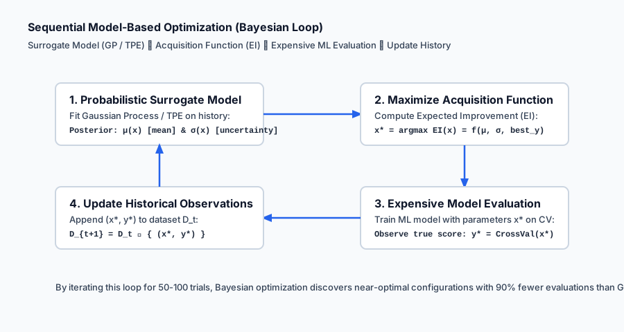
Bayesian Optimization treats hyperparameter tuning as a sequential decision problem:
- Historical Dataset:
H_t = { (theta_1, y_1), (theta_2, y_2), ..., (theta_t, y_t) }of past configurations and their cross-validation scores. - Surrogate Model: A probabilistic regression model (typically a Gaussian Process or Tree-structured Parzen Estimator) that fits
H_tto predict:- Expected score (Mean):
mu(theta) - Epistemic uncertainty (Standard Deviation):
sigma(theta)
- Expected score (Mean):
- Acquisition Function: A cheap mathematical function
alpha(theta)that scores candidate points based onmu(theta)andsigma(theta). - Next Point Selection: Solve
theta_{t+1} = argmax_{theta in Theta} alpha(theta)(cheaply optimized via numerical methods). - Evaluate & Update: Train the true model with
theta_{t+1}, recordy_{t+1}, append toH_{t+1}, and repeat.
4. The Expected Improvement (EI) Acquisition Function
For a maximization objective (e.g. classification accuracy), let y^+ = max_{i=1}^t y_i be the best score observed so far.
The improvement of a new candidate theta is:
I(theta) = max(0, f(theta) - y^+ - xi)
Where xi >= 0 is an exploration parameter.
Under a Gaussian Process surrogate f(theta) ~ N(mu(theta), sigma^2(theta)), the Expected Improvement has an exact closed-form analytical expression:
EI(theta) = E[ I(theta) ] = (mu(theta) - y^+ - xi) * Phi(Z) + sigma(theta) * phi(Z) if sigma(theta) > 0
EI(theta) = 0 if sigma(theta) == 0
Where:
Z = (mu(theta) - y^+ - xi) / sigma(theta)Phi(Z)is the standard Normal Cumulative Distribution Function (CDF).phi(Z)is the standard Normal Probability Density Function (PDF).
Let us dissect the two terms of Expected Improvement:
- Exploitation Term
(mu - y^+ - xi) * Phi(Z): High when the surrogate predicts a high average scoremu(theta). - Exploration Term
sigma(theta) * phi(Z): High when the surrogate has high uncertaintysigma(theta)(unexplored regions of hyperparameter space).
5. Multi-Fidelity Pruning: Successive Halving and Hyperband
Why train 500 trees if a bad configuration (e.g. learning_rate = 10.0) diverges after 10 trees?
Round 0: Start 64 configurations ➔ Train for 10 iterations ➔ Evaluate validation loss.
Round 1: Keep top 32 configurations ➔ Train for 20 iterations.
Round 2: Keep top 16 configurations ➔ Train for 40 iterations.
Round 3: Keep top 8 configurations  ➔ Train for 80 iterations.
Round 4: Keep top 4 configurations  ➔ Train for 160 iterations.
Round 5: Top 2 configurations       ➔ Train for 320 iterations.
Successive Halving discards the worst-performing 50% of candidates at each milestone, focusing compute exclusively on promising configurations. Hyperband wraps Successive Halving across varying initial exploration budgets.
An everyday analogy
Think of hyperparameter tuning as tuning a high-performance race car:
- Model Parameters (The Driver’s Steering): The steering wheel and pedals respond dynamically to the road conditions during the race (fitting the data).
- Hyperparameters (The Mechanical Setup): Gear ratios, tire compound, wing downforce angle, and suspension stiffness are configured in the garage before the race starts.
- Grid Search (The Inflexible Mechanic): The mechanic tests every possible tire with every possible wing angle on a spreadsheet. By the time they finish 1,000 tests, the race season is over.
- Random Search (The Dynamic Tester): The mechanic tests diverse combinations across the full RPM band, quickly discovering that downforce is the single critical factor for this track.
- Bayesian Optimization (The Telemetry AI): The telemetry system analyzes lap times from previous runs, predicts the optimal downforce/gear combination, and dials in the championship setup in 10 test laps.
Examples in practice
Let us visualize the spatial exploration efficiency of Grid vs Random vs Bayesian Search:
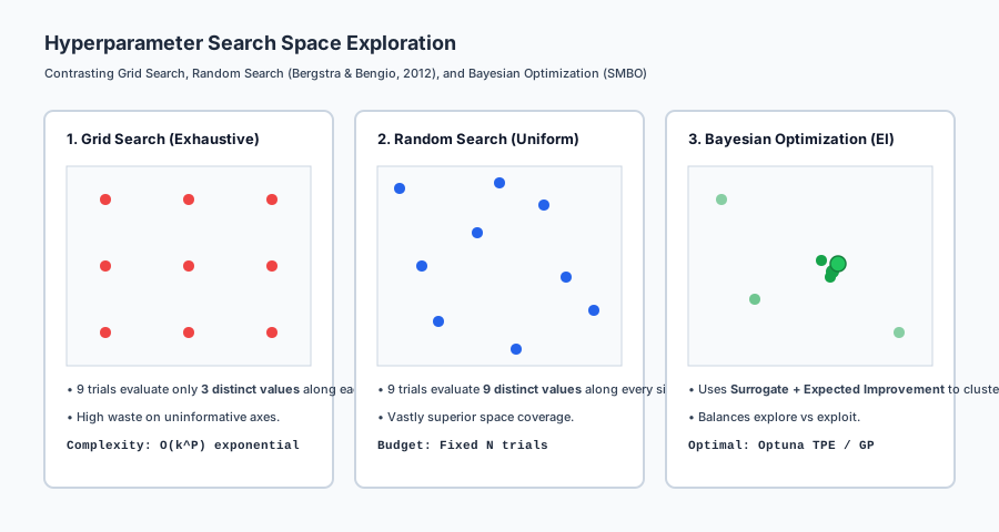
The diagram illustrates how Random Search covers more unique parameter values, while Bayesian Optimization clusters trials around the global optimum.
Below is the cyclical flow of Sequential Model-Based Optimization (SMBO):
Let us examine real Python code performing Randomized Search with cross-validation on a Random Forest:
import numpy as np
from scipy.stats import randint, uniform
from sklearn.datasets import load_breast_cancer
from sklearn.ensemble import RandomForestClassifier
from sklearn.model_selection import RandomizedSearchCV, StratifiedKFold
from sklearn.metrics import accuracy_score, classification_report

# 1. Load Data
cancer = load_breast_cancer()
X, y = cancer.data, cancer.target

# 2. Define Continuous and Discrete Parameter Distributions
param_distributions = {
    "n_estimators": randint(50, 300),
    "max_depth": randint(3, 12),
    "min_samples_split": randint(2, 10),
    "min_samples_leaf": randint(1, 6),
    "max_features": ["sqrt", "log2", None]
}

# 3. Configure Randomized Search with 5-Fold Stratified CV
cv = StratifiedKFold(n_splits=5, shuffle=True, random_state=42)

random_search = RandomizedSearchCV(
    estimator=RandomForestClassifier(random_state=42),
    param_distributions=param_distributions,
    n_iter=30, # 30 random configurations (vastly faster than 5^5 = 3125 grid)
    scoring="accuracy",
    cv=cv,
    n_jobs=-1,
    random_state=42
)

random_search.fit(X, y)

# 4. Inspect Results
print("=== Hyperparameter Tuning Benchmark ===")
print(f"Best 5-Fold CV Score: {random_search.best_score_ * 100:.2f}%")
print("Best Hyperparameters Found:")
for k, v in random_search.best_params_.items():
    print(f"• {k:20s}: {v}")
Implications: security, privacy, performance, scalability, and cost
| Dimension | Characteristic | Practical Implication |
|---|---|---|
| Search Space Budget | Exponential scaling with parameter count. | In high dimensions (P > 8), exhaustive Grid Search is strictly forbidden in production; use Random Search or Optuna. |
| Optimization Leakage | Validation set overfitting. | Running 10,000 trials on a small validation set selects a model that overfit validation noise. Always keep an untouched final test set. |
| Compute Cost & Parallelism | Embarrassingly parallel trials. | Random Search trials are 100% independent and scale linearly across distributed clusters (Ray Tune / Dask). |
| Denial of Service Risks | User-controlled grid configurations. | Web APIs accepting tuning requests must limit n_iter and memory limits to prevent server resource starvation. |
Alternatives: free, open source, and commercial
| Tool / Framework | Methodology | License / Cost | Best Used For |
|---|---|---|---|
scikit-learn (RandomizedSearchCV) | Uniform distribution sampling | Free, BSD Open Source | Baseline tuning directly within scikit-learn workflows. |
Optuna | Tree-structured Parzen Estimator (TPE) + Pruning | Free, MIT Open Source | State-of-the-art Python Bayesian optimization and automated trial pruning. |
Ray Tune | Distributed Hyperband / ASHA | Free, Apache 2.0 | Multi-node, multi-GPU distributed hyperparameter search at scale. |
Weights & Biases Sweeps | Cloud-managed Bayesian tuning | Free tier / Commercial | Experiment tracking and hyperparameter sweeps with web dashboard. |
Comparison with related concepts
| Characteristic | Grid Search | Random Search | Bayesian Optimization (SMBO) |
|---|---|---|---|
| Search Logic | Exhaustive Cartesian grid | Independent random sampling | Probabilistic surrogate + Expected Improvement |
| Sample Efficiency | Very Low (O(k^P)) | High (Covers all axes) | Ultra-High (Focuses near optimum) |
| Parallelizability | Embarrassingly parallel | Embarrassingly parallel | Sequential (or batched async) |
| Setup Complexity | Trivial | Trivial | Requires surrogate configuration |
| Continuous Spaces | Requires manual discretization | Natural sampling | Natural continuous modeling |
When to use it — and when not to
When to USE Systematic Hyperparameter Tuning:
- Final Model Polishing Before Production: To squeeze the final 2–5% accuracy out of a validated feature set.
- Tuning Complex Gradient Boosters (XGBoost/LightGBM): Where learning rate, tree depth, and regularization interact strongly.
- Constrained Inference Latency: To find the smallest
max_depthandn_estimatorsthat still satisfies business accuracy requirements.
When NOT to use Heavy Hyperparameter Tuning:
- Early Exploratory Data Analysis: Don’t waste 4 hours tuning hyperparameters on a dirty dataset with raw un-engineered features.
- Small Datasets with High Noise (
N < 200): Heavy tuning will overfit the validation folds; use a robust default Random Forest instead. - Linear Models with Convex Objectives: Ridge regression has a single hyperparameter
alphaeasily solved via analytical generalized cross-validation (RidgeCV).
Knowledge check
- Parameter vs Hyperparameter: Parameters are fitted by training data; hyperparameters control algorithm capacity.
- Low Effective Dimensionality: Random search evaluates more distinct values of the important parameters than Grid Search.
- Bayesian Optimization: Combines a surrogate model (
mu, sigma) with an acquisition function (Expected Improvement). - Optimization Leakage: Excessive tuning on a validation set overfits validation noise; hold out an untouched test set.
Hands-on exercise
In this hands-on exercise, you will implement analytical Expected Improvement (EI) and evaluate parameter combinations on a synthetic objective.
import numpy as np
from scipy.stats import norm

# Step 1: Implement Expected Improvement
def expected_improvement(mu, sigma, current_best, xi=0.01):
    ei = np.zeros_like(mu)
    valid = sigma > 1e-9
    improvement = mu[valid] - current_best - xi
    Z = improvement / sigma[valid]
    ei[valid] = improvement * norm.cdf(Z) + sigma[valid] * norm.pdf(Z)
    return ei

# Step 2: Compare 3 Candidate Points from a Surrogate Model
# Current Best Score = 0.85
current_best = 0.85

# Candidate A: High mean, low uncertainty (Exploitation)
# Candidate B: Moderate mean, high uncertainty (Exploration)
# Candidate C: Low mean, low uncertainty (Sub-optimal)
candidates_mu = np.array([0.88, 0.83, 0.70])
candidates_sigma = np.array([0.02, 0.12, 0.01])

ei_scores = expected_improvement(candidates_mu, candidates_sigma, current_best, xi=0.01)

print("=== Bayesian Optimization Candidate Selection ===")
for name, mu, sig, ei in zip(["A (Exploit)", "B (Explore)", "C (Sub-optimal)"], candidates_mu, candidates_sigma, ei_scores):
    print(f"Candidate {name:15s}: Mean={mu:.2f}, Sigma={sig:.2f} ➔ Expected Improvement = {ei:.5f}")

best_candidate = np.argmax(ei_scores)
print(f"\nNext Point Selected to Evaluate: Candidate {best_candidate} (Index {best_candidate})")
Expected output
=== Bayesian Optimization Candidate Selection ===
Candidate A (Exploit)    : Mean=0.88, Sigma=0.02 ➔ Expected Improvement = 0.02052
Candidate B (Explore)    : Mean=0.83, Sigma=0.12 ➔ Expected Improvement = 0.02868
Candidate C (Sub-optimal): Mean=0.70, Sigma=0.01 ➔ Expected Improvement = 0.00000

Next Point Selected to Evaluate: Candidate 1 (Index 1)
Validate your work
- Confirm that Candidate B (Explore) receives a higher EI score than Candidate A due to high epistemic uncertainty
sigma = 0.12. - Confirm that Candidate C receives an EI of
0.00000. - Run
RandomizedSearchCVon a Random Forest and verify that 5-fold CV accuracy improves over the un-tuned default.
Troubleshooting
- EI Function Returning NaN: Ensure you handle
sigma == 0by returning0.0. - Search Running Out of Memory: Reduce
n_jobsif memory is exhausted during parallel cross-validation.
Common mistakes
- Running Grid Search on Continuous Parameters: Use log-uniform distributions (
loguniform(1e-4, 1e-1)) with Random Search instead. - Evaluating Tuning on the Test Set: Strictly separate train/validation folds from the final test holdout.
Practice assignment
- Implement Upper Confidence Bound (UCB) Acquisition Function:
Write
compute_ucb(mu, sigma, kappa=2.0)whereUCB = mu + kappa * sigma. Compare the candidate selected by UCB vs Expected Improvement. - Implement Hyperparameter Successive Halving: Write a Python loop that trains 16 Random Forest models for 10 trees, evaluates validation accuracy, keeps the top 8 models, trains them to 20 trees, and repeats until 1 champion model remains.
Extension challenge
Build a Mini-Optuna Bayesian Optimizer from Scratch:
- Implement a 1D Gaussian Process Regressor with an RBF kernel from first principles in NumPy.
- Optimize a non-convex black-box function
f(x) = sin(3x) + 0.5xusing the Bayesian Optimization loop with Expected Improvement for 15 iterations. - Plot the true function, the GP surrogate posterior mean and 95% confidence bounds, and the acquisition function at each step.
Quiz
Q1. What is the fundamental difference between a model parameter and a hyperparameter?
- Parameters (e.g. tree split thresholds, linear weights w) are learned automatically from training data; hyperparameters (e.g. max_depth, learning_rate, n_estimators) are configured before training to control capacity and regularization
- Parameters are for classification; hyperparameters are for regression
- Parameters are integers; hyperparameters are floating-point numbers
- There is no difference
Show answer
Answer: A. Parameters (e.g. tree split thresholds, linear weights w) are learned automatically from training data; hyperparameters (e.g. max_depth, learning_rate, n_estimators) are configured before training to control capacity and regularization
Parameters are internal to the model and optimized directly by the training algorithm. Hyperparameters are external knobs set by the engineer to guide optimization and regularize model capacity.
Q2. Why does Random Search mathematically outperform Grid Search for the same total number of trials (Bergstra & Bengio, 2012)?
- Because most machine learning problems have "low effective dimensionality": only 1 or 2 hyperparameters truly drive performance. Grid search wastes trials testing repeated values along uninformative axes, while Random Search tests N distinct values for every single parameter
- Because Random Search uses GPU acceleration
- Because Random Search always finds the global minimum
- Because Grid Search cannot evaluate integer parameters
Show answer
Answer: A. Because most machine learning problems have "low effective dimensionality": only 1 or 2 hyperparameters truly drive performance. Grid search wastes trials testing repeated values along uninformative axes, while Random Search tests N distinct values for every single parameter
If only learning_rate matters and max_depth is secondary, a 9-trial grid search tests only 3 distinct learning rates. A 9-trial random search tests 9 distinct learning rates, providing 3x better coverage of the critical dimension.
Q3. What are the two core components of a Bayesian Optimization system?
- A Surrogate Model (e.g. Gaussian Process or Tree-structured Parzen Estimator) that models the objective function and uncertainty, and an Acquisition Function (e.g. Expected Improvement) that guides where to sample next
- A linear regression model and a random number generator
- A neural network and a confusion matrix
- A clustering algorithm and a decision tree
Show answer
Answer: A. A Surrogate Model (e.g. Gaussian Process or Tree-structured Parzen Estimator) that models the objective function and uncertainty, and an Acquisition Function (e.g. Expected Improvement) that guides where to sample next
Bayesian optimization uses a probabilistic surrogate model to estimate mean performance mu(x) and uncertainty sigma(x), and an acquisition function to balance exploration (high uncertainty) vs exploitation (high mean).
Q4. In the Expected Improvement (EI) acquisition function, what does the parameter xi >= 0 control?
- The trade-off between exploration and exploitation: larger xi favors exploration of high-uncertainty regions, while xi = 0 favors exploiting near the current best observation
- The learning rate of the booster
- The number of cross-validation folds
- The random seed
Show answer
Answer: A. The trade-off between exploration and exploitation: larger xi favors exploration of high-uncertainty regions, while xi = 0 favors exploiting near the current best observation
The parameter xi specifies the minimum improvement over the current best score required to be considered attractive, shifting search priority towards high-variance unexplored parameter space.
Q5. What is Successive Halving (and its extension Hyperband)?
- A multi-fidelity bandit algorithm that starts many candidate configurations on small resource budgets (e.g. 10 epochs or 1,000 samples), evaluates them, and promotes only the top 50% to progressively larger budgets
- A method that cuts feature count in half
- A binary search over learning rates
- A tree pruning algorithm
Show answer
Answer: A. A multi-fidelity bandit algorithm that starts many candidate configurations on small resource budgets (e.g. 10 epochs or 1,000 samples), evaluates them, and promotes only the top 50% to progressively larger budgets
Successive Halving evaluates dozens of configurations cheaply on small subsets/epochs, quickly killing poor parameter combinations and allocating full compute budgets only to top performers.
Q6. What is the recommended tuning hierarchy for Gradient Boosted Trees (XGBoost / LightGBM)?
- 1. Fix learning_rate (e.g. 0.1) and find optimal n_estimators via early stopping; 2. Tune tree structure (max_depth / max_leaf_nodes, min_child_samples); 3. Tune stochastic sampling (subsample, colsample_bytree); 4. Tune regularization (reg_alpha, reg_lambda); 5. Lower learning_rate (0.01) and retrain
- 1. Tune random_state; 2. Tune thread count; 3. Run grid search
- 1. Tune lambda; 2. Set max_depth=50
- 1. Tune batch size; 2. Train for 1 epoch
Show answer
Answer: A. 1. Fix learning_rate (e.g. 0.1) and find optimal n_estimators via early stopping; 2. Tune tree structure (max_depth / max_leaf_nodes, min_child_samples); 3. Tune stochastic sampling (subsample, colsample_bytree); 4. Tune regularization (reg_alpha, reg_lambda); 5. Lower learning_rate (0.01) and retrain
Systematic tuning starts by locking in tree capacity and early stopping at a moderate learning rate, tuning structural and sampling regularizers, and finally reducing learning rate with increased trees for a final accuracy boost.
Q7. What is "Optimization Leakage" (overfitting the validation set during hyperparameter tuning)?
- When thousands of hyperparameter configurations are evaluated on a small validation set, the search eventually picks a configuration that memorized the validation noise rather than learning generalizable patterns
- When test labels leak into the training set
- When missing values are imputed before scaling
- When features are correlated
Show answer
Answer: A. When thousands of hyperparameter configurations are evaluated on a small validation set, the search eventually picks a configuration that memorized the validation noise rather than learning generalizable patterns
Just as model parameters can overfit the training set, hyperparameter search algorithms can overfit the validation set if too many configurations are tested without a completely isolated holdout test set.
Q8. Why is it dangerous to tune hyperparameters using only training set accuracy?
- The search will always select the most complex, unconstrained model (e.g. max_depth=None, min_samples_split=2, n_estimators=10000), resulting in 100% training accuracy but catastrophic test-set overfitting
- Training accuracy cannot be computed for decision trees
- Grid search crashes if cross-validation is disabled
- Hyperparameters only affect test accuracy
Show answer
Answer: A. The search will always select the most complex, unconstrained model (e.g. max_depth=None, min_samples_split=2, n_estimators=10000), resulting in 100% training accuracy but catastrophic test-set overfitting
Training accuracy monotonically favors maximum complexity. Hyperparameters MUST be evaluated on held-out cross-validation folds to measure true generalization.
Glossary
- Hyperparameter
- A configuration external to the model whose value is set before the learning process begins, dictating model capacity, optimization dynamics, and regularization.
- Grid Search
- An exhaustive hyperparameter optimization strategy that trains and evaluates models across all combinations in a predefined discrete Cartesian product grid.
- Random Search
- A hyperparameter optimization method that samples parameter configurations randomly from specified statistical distributions, providing superior coverage of continuous spaces.
- Bayesian Optimization
- A sequential design strategy for global optimization that builds a probabilistic surrogate model of the objective function to intelligently select the most promising evaluation points.
- Surrogate Model
- A computationally cheap probabilistic approximation (e.g. Gaussian Process, Tree-structured Parzen Estimator) of the true expensive objective function.
- Acquisition Function
- A mathematical function (such as Expected Improvement or Upper Confidence Bound) that guides search exploration by quantifying the utility of sampling a candidate hyperparameter point.
- Expected Improvement (EI)
- An acquisition function that measures the expected magnitude of performance gain over the current best observed score, integrating over the surrogate posterior uncertainty.
- Successive Halving
- An early-stopping resource allocation algorithm that trains a pool of configurations on minimal resources, progressively pruning the bottom half and promoting top candidates.
- Hyperband
- A bandit-based hyperparameter optimization framework that extends Successive Halving across varying initial resource allocations to resolve the exploration vs exploitation trade-off.
- Optimization Leakage
- The phenomenon where hyperparameter tuning overfits a specific validation fold due to excessive trials, necessitating an untouched external test set for final audit.
Sources and further reading
- Random Search for Hyper-Parameter Optimization — Journal of Machine Learning Research (James Bergstra and Yoshua Bengio) (accessed 2026-08-29)
- Practical Bayesian Optimization of Machine Learning Algorithms — NeurIPS (Jasper Snoek, Hugo Larochelle, Ryan P. Adams) (accessed 2026-08-29)
- Hyperband: A Novel Bandit-Based Approach to Hyperparameter Optimization — Journal of Machine Learning Research (Lisha Li, Kevin Jamieson, et al.) (accessed 2026-08-29)
Kept in this browser, no account needed. Your progress page turns the whole record into one link you can bookmark or open on another device.