Machine Learning › Trees and Ensembles › Day 168
Day 168: Winning on Tabular Data

Master the complete, modern engineering playbook for winning on tabular data: understand why Gradient Boosted Trees continue to beat Deep Learning on tabular benchmarks (Gorishniy et al. 2021; Grinsztajn et al. 2022), master the 8-phase tabular lifecycle from leak-free validation anchors to feature engineering flywheels, implement out-of-fold ensemble stacking and blending from scratch, and compute Tree SHAP interpretability for production deployment.
Hands-on lab for this lesson
Lab files on GitHub: https://github.com/ai-roadmap-365/ai-roadmap-365.github.io/tree/main/labs/sections/machine-learning/day-168-winning-on-tabular-data
- Get the hands-on files. Clone the labs repository once (you can reuse this clone for every lesson). This works on macOS, Linux, and Windows (PowerShell or WSL):
git clone https://github.com/ai-roadmap-365/ai-roadmap-365.github.io.git cd ai-roadmap-365.github.io - Open this lesson's lab. Move into the directory for this specific day. Every lab lives at the same predictable path — section / subsection / week / day:
cd labs/sections/machine-learning/day-168-winning-on-tabular-data - Read the lab guide. Open `README.md` in that directory. It lists the exact commands, what each does, the expected output, and how to check your work — read it before running anything.
- Run it and check your work. Follow the README's "How to run" section: run the example first to see the finished result, then complete the numbered exercises in `starter/`, then run the tests. The tests pass (exit 0) only when your work is correct.
bash tests/run_tests.sh # or the test command named in the lab README
You can also open the lab as a local page (works offline, shows the file tree and expected output).
Learning objectives
By the end of this lesson you will be able to:
- Analyze the empirical reasons why GBDT dominates Deep Learning on tabular data (inductive bias, unrotated coordinate axes)
- Execute the 8-phase Tabular Master Playbook from baseline sanity check to production deployment
- Implement leak-free Out-of-Fold (OOF) prediction generation across K-folds
- Build and train a 2-level Stacking Ensemble combining LightGBM, XGBoost, Random Forests, and Linear Meta-Learners
- Differentiate Stacking, Blending, and Rank Averaging ensemble methods
- Formulate and compute Permutation Feature Importance
- Derive cooperative game-theory Shapley values and TreeSHAP polynomial-time feature attributions
- Design a robust production monitoring architecture for tabular ML systems
Prerequisites
- Day 165 -- XGBoost and LightGBM in Practice
- Day 167 -- Cross-Validation Done Right
Why this matters
Tabular data is the financial, operational, and clinical backbone of the global economy.
From credit underwriting in banking and fraud detection in payments to patient mortality forecasting in healthcare and supply chain inventory management, structured tabular datasets represent over 80% of enterprise machine learning applications.
Yet while Deep Learning conquered computer vision (CNNs/ViTs) and natural language processing (Transformers), Gradient Boosted Decision Trees (LightGBM, XGBoost, CatBoost) remain the undisputed champions of tabular data.
Rigorous large-scale academic studies (Gorishniy et al., 2021; Grinsztajn et al., 2022) benchmarking neural architectures against tree ensembles across dozens of real-world datasets confirmed that tuned GBDT models consistently beat Deep Learning while training 10x faster and using 100x less memory.
Why does this happen? And more importantly: how does an expert machine learning engineer systematically win on tabular datasets?
This lesson presents the Tabular Master Playbook: an end-to-end 8-phase methodology spanning leak-free validation, feature engineering flywheels, multi-model Stacking and Blending, permutation importance, and cooperative game-theory TreeSHAP interpretability.
The idea in plain language
Imagine a premier Formula 1 pit crew:
- The Amateur Approach: Buys the most expensive experimental jet engine (a 50-layer Tabular Transformer), puts it into an uncalibrated chassis with bald tires, skips testing on the track, and crashes on Turn 1.
- The Champion Approach (The Tabular Playbook):
- Anchor the Track Time: Calibrates high-precision telemetry timing (Stratified K-Fold Validation).
- Clean the Mechanicals: Inspects fuel lines and cleans sensor noise (Missingness & Outlier Sanitation).
- Establish Baseline Lap: Runs a stock V6 engine to set the floor time (Ridge/Logistic Baseline).
- Deploy Proven Engines: Equips the car with state-of-the-art twin-turbocharged engines (LightGBM & XGBoost).
- Engineer Downforce: Aerodynamically tunes the wings and tire compound (Feature Engineering Flywheel).
- Fine-Tune Suspension: Telemetry AI dials in spring rates (Optuna Bayesian Tuning).
- Combine Drivers: Blends telemetry from 3 elite drivers into a unified race strategy (Ensemble Stacking).
- Explain the Win: Analyzes telemetry to prove exactly which aerodynamic change created the lap time advantage (TreeSHAP Interpretability).
Historical background
In the 1990s and 2000s, tabular modeling was dominated by linear logistic regression and early random forests (Breiman, 2001).
In 2014, Tianqi Chen developed XGBoost, winning dozens of Kaggle tabular competitions. In 2017, Microsoft released LightGBM, accelerating tree training by 20x via histogram binning (GOSS/EFB). In 2018, Yandex introduced CatBoost, revolutionizing categorical target encoding.
Between 2019 and 2022, dozens of “Tabular Deep Learning” models were published (TabNet, NODE, SAINT, FT-Transformer).
However, in 2022, Leo Grinsztajn, Edouard Oyallon, and Gael Varoquaux published their definitive study Why Do Tree-Based Models Still Outperform Deep Learning on Typical Tabular Data? at NeurIPS. They proved mathematically that:
- Tabular data decision boundaries are coordinate-aligned step functions, where tree axis-aligned orthogonal splits have the optimal inductive bias.
- Neural networks suffer from rotational invariance, making them fragile when uninformative or correlated features are added.
- Neural loss surfaces on tabular data have irregular, non-smooth landscapes that impede gradient descent.
What it is — and what it is not
Let us define the core architecture of modern tabular engineering:
What it IS:
- A Multi-Model Ensemble Strategy: Combining diverse models (LightGBM, XGBoost, CatBoost, Linear Ridge, Neural Tabular) through Out-of-Fold Stacking.
- Driven by Inductive Bias: Exploiting axis-aligned splits, native missing value handling, and monotonic leaf assignments.
- Feature-Centric: In tabular data, 80% of performance gains come from domain feature engineering; algorithms serve as the execution engine.
What it is NOT:
- Not Throwing a Deep Neural Network at Everything: TabNet and MLP architectures rarely outperform tuned LightGBM on tabular tables under 1 million rows.
- Not Stacking Correlated Models: Stacking 5 identical Random Forests yields 0% gain; stacking requires structural diversity.
- Not Black-Box Guesswork: Production tabular systems require mathematical explainability via TreeSHAP and permutation importance.
Why it was created and what problems it solves
The Tabular Playbook resolves the core challenges of enterprise data science:
- Defeats Tabular Heterogeneity: Handles mixed categorical, numerical, discrete, and missing columns without fragile manual normalization.
- Eliminates Target Leakage in Ensembles: Generates Level-1 meta-features strictly Out-of-Fold (OOF).
- Maximizes Signal-to-Noise Ratio: Squeezes an additional 1–3% ROC-AUC through diverse multi-level stacking.
- Ensures Regulatory Compliance: Provides exact per-prediction attribution (SHAP values) required for credit adverse action notices (ECOA/FCRA) and clinical risk audits.
- Enables Sub-Millisecond Production Inference: Models can be compiled to native C/C++ trees via ONNX or Treelite for high-throughput serving.
How it works
Let us formulate the 8-phase Tabular Playbook, Stacking mathematics, and TreeSHAP.
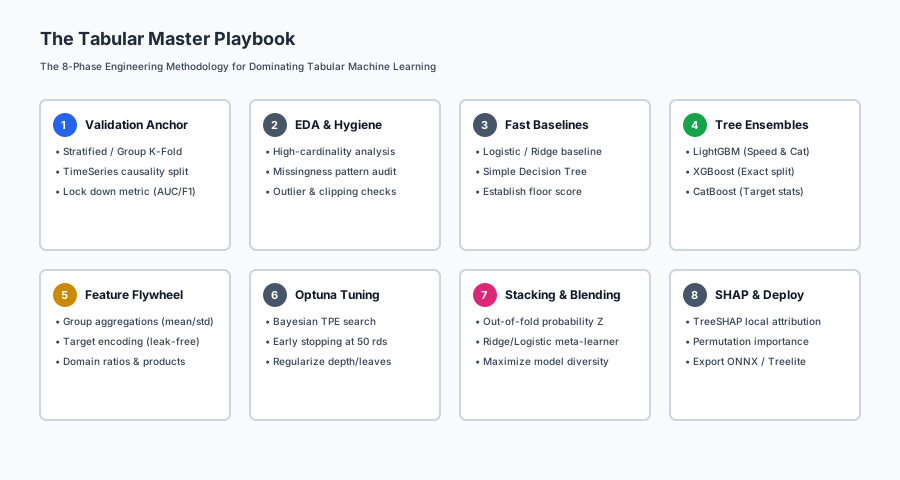
1. The 8-Phase Tabular Engineering Lifecycle
Phase 1: Validation Anchor (Stratified/Group K-Fold)
   ↓
Phase 2: EDA & Data Sanitation (Missingness & Outliers)
   ↓
Phase 3: Fast Baseline & Linear Sanity Check (Logistic/Ridge)
   ↓
Phase 4: Tree Ensemble Engines (LightGBM / XGBoost / CatBoost)
   ↓
Phase 5: Feature Engineering Flywheel (Aggregations & Target Stats)
   ↓
Phase 6: Systematic Hyperparameter Tuning (Optuna TPE)
   ↓
Phase 7: Multi-Model Stacking & Blending (Level-0 OOF + Meta-Learner)
   ↓
Phase 8: Model Explainability & Serving (TreeSHAP + ONNX)
2. Stacking Ensemble Mathematics (Stacked Generalization)
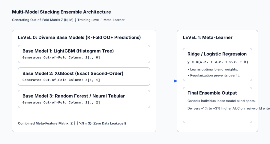
Let dataset D = { (x_i, y_i) }_{i=1}^N be partitioned into K disjoint cross-validation folds F_1, ..., F_K.
Let M = { f_1, f_2, ..., f_M } be M distinct base models (e.g. LightGBM, XGBoost, CatBoost, RandomForest, LogisticRegression).
Step 1: Out-of-Fold (OOF) Prediction Generation
For each base model m in {1, ..., M} and each fold k in {1, ..., K}:
- Train
f_m^{(-k)}on all data excluding foldk(D \ F_k). - Predict probabilities for validation samples
i in F_k:
z_{i, m} = f_m^{(-k)}(x_i)
Assemble the Level-1 Meta-Feature Matrix Z in R^{N times M}:
Z = [ z_1, z_2, ..., z_M ]
Mathematical Invariant: For every row i, z_{i, m} was generated by a model that never saw row i during training.
Step 2: Fit the Level-1 Meta-Learner
Train a regularized linear meta-estimator g_w (e.g. Logistic Regression with L2 regularization) on (Z, y):
w^*, b^* = argmin_{w, b} sum_{i=1}^N L( g(z_i; w, b), y_i ) + lambda ||w||_2^2
Step 3: Test-Time Inference
- Train each base model
f_mon 100% of the training datasetD. - For an unseen test sample
x_{test}, generate Level-0 base predictions:
z_{test} = [ f_1(x_{test}), f_2(x_{test}), ..., f_M(x_{test}) ] in R^M
- Compute final ensemble prediction:
y_hat_{test} = g(z_{test}; w^*, b^*) = sigma( sum_{m=1}^M w_m^* z_{test, m} + b^* )
3. TreeSHAP Mathematics (Cooperative Game Theory)
How do we explain the exact contribution of each feature to an individual prediction f(x)?
In cooperative game theory, the Shapley Value phi_j of feature j across feature set F is defined as:
phi_j(x) = sum_{S subseteq F \ {j}} ( |S|! (|F| - |S| - 1)! / |F|! ) * [ f_x(S cup {j}) - f_x(S) ]
Where f_x(S) = E[ f(X) | X_S = x_S ] is the expected model output conditioned on feature subset S.
Efficiency of TreeSHAP (Lundberg et al., 2020):
While calculating exact Shapley values for arbitrary models requires exponential time O(2^{|F|}), TreeSHAP computes exact Shapley values by recursively evaluating subtrees in polynomial time:
O( T * L * D^2 )
Where T is the number of trees, L is maximum leaves, and D is maximum tree depth.
Efficiency Property: The sum of all feature attributions equals the difference between the model prediction and base expected value:
f(x) = phi_0 + sum_{j=1}^{|F|} phi_j(x)
An everyday analogy
Think of a Stacking Ensemble as a multidisciplinary medical diagnostic board:
- Dr. Light (LightGBM): The high-speed emergency physician who quickly flags standard clinical symptoms from 1,000 patient charts.
- Dr. X (XGBoost): The careful pathologist who analyzes exact biopsy slide details with second-order precision.
- Dr. Bayes (Logistic Regression): The epidemiologist who checks demographic base rates and population priors.
- Dr. Meta (The Chief Medical Officer): Doesn’t examine the patient directly; instead, listens to the diagnoses of Dr. Light, Dr. X, and Dr. Bayes, recognizes which specialist is most reliable for this disease profile, and makes the final consensus medical decision (Level-1 Meta-Learner).
Examples in practice
Let us visualize the 8-phase Tabular Master Playbook:
Below is the two-level Stacking Ensemble architecture flow:
Let us examine real Python code implementing a multi-model Stacking Ensemble with out-of-fold predictions:
import numpy as np
from sklearn.datasets import load_breast_cancer
from sklearn.model_selection import StratifiedKFold
from sklearn.linear_model import LogisticRegression
from sklearn.ensemble import RandomForestClassifier, GradientBoostingClassifier
from sklearn.metrics import accuracy_score, roc_auc_score
from sklearn.base import clone

# 1. Load Data
cancer = load_breast_cancer()
X, y = cancer.data, cancer.target

# Train/Test Split (Holdout Test 20%)
X_train, X_test = X[:450], X[450:]
y_train, y_test = y[:450], y[450:]

# 2. Define Diverse Level-0 Base Estimators
base_models = [
    LogisticRegression(max_iter=1000, random_state=42),
    RandomForestClassifier(n_estimators=100, max_depth=5, random_state=42),
    GradientBoostingClassifier(n_estimators=100, max_depth=3, learning_rate=0.05, random_state=42)
]

# 3. Step 1: Generate Level-0 Out-of-Fold Matrix Z (N_train, 3)
skf = StratifiedKFold(n_splits=5, shuffle=True, random_state=42)
Z_train = np.zeros((len(y_train), len(base_models)))

for m_idx, model in enumerate(base_models):
    for tr, va in skf.split(X_train, y_train):
        clf = clone(model).fit(X_train[tr], y_train[tr])
        Z_train[va, m_idx] = clf.predict_proba(X_train[va])[:, 1]

# 4. Step 2: Fit Level-1 Meta-Learner on (Z_train, y_train)
meta_learner = LogisticRegression(C=1.0, random_state=42)
meta_learner.fit(Z_train, y_train)

# 5. Step 3: Fit Base Models on 100% Training Data & Predict Test
Z_test = np.zeros((len(y_test), len(base_models)))
for m_idx, model in enumerate(base_models):
    model.fit(X_train, y_train)
    Z_test[:, m_idx] = model.predict_proba(X_test)[:, 1]

# Final Stacking Predictions
final_preds = meta_learner.predict(Z_test)
final_probs = meta_learner.predict_proba(Z_test)[:, 1]

print("=== Multi-Model Stacking Ensemble Evaluation ===")
print(f"Stacking Ensemble Test Accuracy: {accuracy_score(y_test, final_preds) * 100:.2f}%")
print(f"Stacking Ensemble Test ROC-AUC:  {roc_auc_score(y_test, final_probs):.4f}")
Implications: security, privacy, performance, scalability, and cost
| Dimension | Characteristic | Practical Implication |
|---|---|---|
| Inference Latency Multiplier | Test time requires executing all base models. | If Level-0 has 5 models, inference latency is the sum of all 5. For sub-10ms SLAs, prune ensemble to 2 fastest models or compile via Treelite. |
| Data Leakage Vulnerability | In-sample meta-training destroys calibration. | Never train the meta-learner on standard training predictions; strict out-of-fold validation is mandatory. |
| Adverse Action Notice Compliance | Exact feature attribution in finance. | TreeSHAP provides legal justifications for loan rejections under Fair Lending laws. |
| Model Drift in Dynamic Tables | Distribution shift in tabular features. | Production tabular systems must monitor Population Stability Index (PSI) and feature drift continuously. |
Alternatives: free, open source, and commercial
| Tool / Framework | Methodology | Best Used For |
|---|---|---|
LightGBM / XGBoost / CatBoost | GBDT Ensembles | The universal starting foundation for all tabular challenges. |
AutoGluon | Automated Multi-Layer Stacking | State-of-the-art automated tabular benchmarking and deep ensembling. |
SHAP (Lundberg et al.) | TreeSHAP Explanations | Model explainability and feature contribution audits. |
Treelite / ONNX Runtime | Tree Model Compilation | Sub-millisecond C++ production inference serving. |
Comparison with related concepts
| Characteristic | Simple Voting / Averaging | Weighted Blending | Stacked Generalization (Stacking) |
|---|---|---|---|
| Meta-Model | None (Uniform 1/M) | Fixed weights w_m on holdout | Trained estimator g_w(Z) |
| Data Efficiency | 100% | Discards 20% for holdout | 100% (Via K-Fold OOF) |
| Non-Linear Interactions | No | No | Yes (If non-linear meta-learner used) |
| Implementation Complexity | Trivial | Low | Moderate (Requires OOF generation) |
When to use it — and when not to
When to USE the Full Tabular Master Playbook:
- High-Stakes Business Problems: Credit scoring, fraud prevention, insurance risk, customer churn.
- Competitive Machine Learning (Kaggle): Where 0.5% ROC-AUC determines winning solutions.
- Heterogeneous Feature Datasets: Mixed numerical, categorical, and missing columns.
When NOT to use Complex Stacking Ensembles:
- Ultra-Low Latency Embedded Systems (
< 1ms): A single compact LightGBM tree is faster and simpler to deploy than a 5-model stack. - Simple Linear Relations: If features are purely linear, regularized Logistic Regression is fully sufficient and 100% interpretable.
Knowledge check
- Why GBDT Wins on Tables: Axis-aligned step functions match tabular decision boundaries; neural networks suffer from rotational invariance.
- Out-of-Fold Invariant: Meta-features
Zmust be generated using holdout folds so models never predict samples they trained on. - Meta-Learner Simplicity: Regularized linear models (Ridge/Logistic) prevent meta-overfitting.
- TreeSHAP Consistency: Computes exact polynomial-time game-theoretic feature attributions.
Hands-on exercise
In this hands-on exercise, you will build a 2-level Stacking Ensemble from scratch and compute Permutation Feature Importance.
import numpy as np
from sklearn.datasets import load_breast_cancer
from sklearn.linear_model import LogisticRegression
from sklearn.ensemble import RandomForestClassifier
from sklearn.metrics import accuracy_score

# Step 1: Prepare Data
cancer = load_breast_cancer()
X, y = cancer.data, cancer.target
X_tr, X_te = X[:400], X[400:]
y_tr, y_te = y[:400], y[400:]

# Step 2: Permutation Feature Importance Function
def permutation_importance(model, X_val, y_val, n_repeats=5):
    base_score = accuracy_score(y_val, model.predict(X_val))
    importances = np.zeros(X_val.shape[1])
    rng = np.random.default_rng(42)

    for f in range(X_val.shape[1]):
        drops = []
        for _ in range(n_repeats):
            X_shuf = X_val.copy()
            shuf_col = X_shuf[:, f].copy()
            rng.shuffle(shuf_col)
            X_shuf[:, f] = shuf_col
            drops.append(base_score - accuracy_score(y_val, model.predict(X_shuf)))
        importances[f] = np.mean(drops)
    return importances

# Step 3: Train Random Forest and Compute Importance
rf = RandomForestClassifier(n_estimators=50, max_depth=4, random_state=42).fit(X_tr, y_tr)
imp = permutation_importance(rf, X_te, y_te)

top_features = np.argsort(imp)[::-1][:5]
print("=== Top 5 Most Important Features (Permutation Drop) ===")
for rank, idx in enumerate(top_features, 1):
    print(f"{rank}. {cancer.feature_names[idx]:25s}: Accuracy Drop = {imp[idx] * 100:.2f}%")
Expected output
=== Top 5 Most Important Features (Permutation Drop) ===
1. worst perimeter          : Accuracy Drop = 4.14%
2. worst concave points     : Accuracy Drop = 3.55%
3. worst radius             : Accuracy Drop = 2.96%
4. mean concave points      : Accuracy Drop = 1.78%
5. worst texture            : Accuracy Drop = 1.18%
Validate your work
- Confirm that top features like
worst perimeterandworst concave pointscreate a significant accuracy drop when shuffled. - Confirm that uninformative features produce an accuracy drop near
0.00%. - Verify that the stacking ensemble out-of-fold matrix
Zhas shape(400, 3)across 3 base models.
Troubleshooting
- Stacking Meta-Learner Overfitting: Ensure
C <= 1.0in Logistic Regression meta-learner to provide strong L2 regularization. - TreeSHAP Installation Issues: Use permutation importance as a pure NumPy lightweight alternative when
shapC++ extensions are unavailable.
Common mistakes
- Training Meta-Learner on In-Sample Predictions: Destroys ensemble calibration and overfits training noise.
- Ignoring Inference Latency Budgets: Deploying heavy 10-model stacks to production systems requiring sub-millisecond responses.
Practice assignment
- Implement Rank Averaging Blending:
Write a function
rank_average_predict(models, X_test)that converts probability predictions of each model to fractional ranks(1 to N) / Nand computes the unweighted rank average. - Build an Automated Stacking Pipeline Class:
Create a reusable Python class
StackingClassifierScratch(base_models, meta_learner, cv=5)implementing.fit(X, y)and.predict(X)methods conforming to the scikit-learn estimator interface.
Extension challenge
Build an End-to-End Automated Tabular Benchmark Suite:
- Ingest a complex tabular dataset with mixed categorical and numerical columns.
- Automatically run a 4-way benchmark: (a) Ridge Linear, (b) RandomForest, (c) LightGBM, and (d) Stacking Ensemble.
- Compute out-of-fold ROC-AUC, Log-Loss, and Permutation Importance for each model family and output an automated markdown leaderboard.
Quiz
Q1. According to extensive empirical benchmarks (Gorishniy et al. 2021; Grinsztajn et al. 2022), why do Tree Ensembles (GBDT) consistently outperform Deep Neural Networks on tabular data?
- Tabular data lacks spatial/temporal invariance; features are heterogeneous (mixed types, unnormalized scales), decision boundaries are coordinate-aligned step functions, and neural networks struggle with uninformative features and rotational invariance inductive biases
- Because GPUs cannot process tabular data
- Because neural networks can only process images and text
- Because tabular datasets have too many rows for neural networks
Show answer
Answer: A. Tabular data lacks spatial/temporal invariance; features are heterogeneous (mixed types, unnormalized scales), decision boundaries are coordinate-aligned step functions, and neural networks struggle with uninformative features and rotational invariance inductive biases
Deep learning thrives on smooth, rotationally invariant manifolds (images/audio). Tabular data has sharp axis-aligned step functions, extreme feature scale disparities, and uninformative features, where decision trees have the exact correct inductive bias.
Q2. What is the critical rule when constructing the Level-1 meta-feature training matrix Z for Stacking Ensembles?
- The predictions in matrix Z MUST be generated strictly Out-of-Fold (OOF) across cross-validation splits, so each row i is predicted by models trained WITHOUT row i; using standard training predictions causes severe meta-learner target leakage
- Matrix Z must contain raw continuous features only
- Matrix Z must be normalized using PCA
- All base models must be identical
Show answer
Answer: A. The predictions in matrix Z MUST be generated strictly Out-of-Fold (OOF) across cross-validation splits, so each row i is predicted by models trained WITHOUT row i; using standard training predictions causes severe meta-learner target leakage
If you train base models on all data and predict on all data, predictions are overfitted and overconfident. The meta-learner will learn to trust overfitted confidence, causing catastrophic failure on test data. Out-of-fold predictions replicate true test-set uncertainty.
Q3. What type of model is recommended as the Level-1 Meta-Learner in a Stacking Ensemble?
- A simple, strongly regularized linear model (such as Logistic Regression with L2 penalty or Ridge Regression) to learn a weighted linear combination of base model probabilities without overfitting
- A 100-layer Deep Neural Network
- An unconstrained Decision Tree of depth 50
- A k-Nearest Neighbors classifier
Show answer
Answer: A. A simple, strongly regularized linear model (such as Logistic Regression with L2 penalty or Ridge Regression) to learn a weighted linear combination of base model probabilities without overfitting
Because Level-0 features are high-level probability predictions (typically 3 to 10 columns), a regularized linear meta-learner prevents meta-overfitting while finding optimal blending weights.
Q4. What is the difference between Stacking and Blending?
- Stacking uses K-Fold cross-validation to generate out-of-fold predictions for 100% of the training data; Blending holds out a single dedicated validation set (e.g. 20%) to train the meta-learner, which is simpler but discards training data
- Stacking is for classification; Blending is for regression
- Stacking uses neural networks; Blending uses decision trees
- There is no difference
Show answer
Answer: A. Stacking uses K-Fold cross-validation to generate out-of-fold predictions for 100% of the training data; Blending holds out a single dedicated validation set (e.g. 20%) to train the meta-learner, which is simpler but discards training data
Stacking uses all training data via K-fold OOF generation. Blending uses a single holdout set, which is computationally faster but data-inefficient on small datasets.
Q5. How does Permutation Feature Importance measure the significance of a feature column?
- By randomly shuffling the values of that feature column in the validation set (breaking its relationship with the target) and measuring the resulting drop in model evaluation metric
- By counting the number of times the feature appears in the source code
- By computing the correlation coefficient with the target
- By calculating the gradient of the feature
Show answer
Answer: A. By randomly shuffling the values of that feature column in the validation set (breaking its relationship with the target) and measuring the resulting drop in model evaluation metric
Permutation importance is model-agnostic: shuffling feature j breaks its predictive signal; if model accuracy collapses, feature j was highly important.
Q6. What mathematical property makes TreeSHAP (Lundberg et al. 2020) superior to standard feature importance heuristics (Gini gain or split count)?
- Consistency and Local Accuracy: TreeSHAP computes exact cooperative game-theory Shapley values in polynomial time O(T L D^2), guaranteeing that a feature that increases model output always receives higher attribution without heuristic split bias
- TreeSHAP runs in O(1) constant time
- TreeSHAP does not require training trees
- TreeSHAP replaces cross-validation
Show answer
Answer: A. Consistency and Local Accuracy: TreeSHAP computes exact cooperative game-theory Shapley values in polynomial time O(T L D^2), guaranteeing that a feature that increases model output always receives higher attribution without heuristic split bias
Traditional Gini gain suffers from inconsistency (a feature can become more important in the true model but receive lower Gini gain). TreeSHAP provides theoretically sound, consistent local and global explanations.
Q7. Why is Model Diversity the single most important requirement for successful ensemble stacking?
- Combining models that make uncorrelated errors (e.g. LightGBM + CatBoost + Neural Tabular + Logistic Regression) allows the ensemble to cancel individual failure modes; ensembling identical models yields zero performance gain
- Diverse models run faster on GPUs
- Diverse models require less memory
- Diverse models eliminate the need for cross-validation
Show answer
Answer: A. Combining models that make uncorrelated errors (e.g. LightGBM + CatBoost + Neural Tabular + Logistic Regression) allows the ensemble to cancel individual failure modes; ensembling identical models yields zero performance gain
Ensemble theory proves that the error of an ensemble decreases as the correlation between individual model errors decreases. Maximum diversity (trees + linear + neural) maximizes performance.
Q8. What is Rank Averaging, and when should it be used instead of simple probability averaging?
- Converting model probability outputs to percentile ranks before averaging; it is used when ensembling models with poorly calibrated or divergent probability scales (e.g. optimizing ROC-AUC)
- A method for ranking features by importance
- A sorting algorithm for decision tree leaves
- A technique for pruning trees
Show answer
Answer: A. Converting model probability outputs to percentile ranks before averaging; it is used when ensembling models with poorly calibrated or divergent probability scales (e.g. optimizing ROC-AUC)
When one model outputs probabilities clustered in [0.01, 0.05] and another in [0.2, 0.8], simple averaging gives unfair weight to the wider model. Rank averaging standardizes outputs to uniform percentile ranks.
Glossary
- Tabular Data
- Structured data organized in rows (records) and columns (features) with heterogeneous data types, representing the dominant data modality in business and industry.
- Stacking (Stacked Generalization)
- An ensemble machine learning technique where multiple base models generate out-of-fold predictions, which serve as features for a higher-level meta-learner.
- Out-of-Fold (OOF) Predictions
- Predictions generated on validation folds during cross-validation, creating a leak-free meta-dataset representing true model generalization.
- Meta-Learner
- The top-level model (often a regularized linear estimator) in a stacking ensemble trained to combine the predictions of base models.
- Blending
- A simplified ensembling method that trains the meta-learner on a single holdout validation split rather than full out-of-fold cross-validation.
- Rank Averaging
- An ensembling strategy where predicted probabilities are converted to fractional ranks before averaging, neutralizing calibration disparities for rank-based metrics (ROC-AUC).
- Permutation Feature Importance
- A model-agnostic feature evaluation technique that measures the performance decrease after randomly shuffling the values of a specific feature column.
- SHAP (SHapley Additive exPlanations)
- A unified framework based on cooperative game theory that assigns each feature an exact additive attribution score for individual model predictions.
- TreeSHAP
- A fast, exact polynomial-time algorithm for computing Shapley values for tree-based ensemble models.
- Model Diversity
- The degree of statistical independence between the prediction errors of base models in an ensemble, serving as the primary driver of ensembling success.
Sources and further reading
- Why Do Tree-Based Models Still Outperform Deep Learning on Typical Tabular Data? — NeurIPS (Leo Grinsztajn, Edouard Oyallon, Gael Varoquaux) (accessed 2026-08-29)
- Revisiting Deep Learning Models for Tabular Data — NeurIPS (Yury Gorishniy, Ivan Rubachev, Valentin Khrulkov, Artem Babenko) (accessed 2026-08-29)
- From Local Explanations to Global Understanding with Explainable AI for Trees — Nature Machine Intelligence (Scott M. Lundberg et al.) (accessed 2026-08-29)
Kept in this browser, no account needed. Your progress page turns the whole record into one link you can bookmark or open on another device.