Machine Learning › Features and Support Vector Machines › Day 169
Day 169: Support Vector Machines

Master the theory and practical mathematics of Support Vector Machines (SVMs): understand geometric margin maximization, primal and dual Quadratic Programming formulations (Cortes & Vapnik, 1995), slack variables and Hinge Loss regularization (C), the revolutionary Kernel Trick (Mercer's Theorem) mapping non-linear data into infinite-dimensional Hilbert spaces with RBF kernels, why feature scaling is strictly mandatory, and when to use LinearSVC vs Kernel SVMs vs Tree Ensembles.
Hands-on lab for this lesson
Lab files on GitHub: https://github.com/ai-roadmap-365/ai-roadmap-365.github.io/tree/main/labs/sections/machine-learning/day-169-support-vector-machines
- Get the hands-on files. Clone the labs repository once (you can reuse this clone for every lesson). This works on macOS, Linux, and Windows (PowerShell or WSL):
git clone https://github.com/ai-roadmap-365/ai-roadmap-365.github.io.git cd ai-roadmap-365.github.io - Open this lesson's lab. Move into the directory for this specific day. Every lab lives at the same predictable path — section / subsection / week / day:
cd labs/sections/machine-learning/day-169-support-vector-machines - Read the lab guide. Open `README.md` in that directory. It lists the exact commands, what each does, the expected output, and how to check your work — read it before running anything.
- Run it and check your work. Follow the README's "How to run" section: run the example first to see the finished result, then complete the numbered exercises in `starter/`, then run the tests. The tests pass (exit 0) only when your work is correct.
bash tests/run_tests.sh # or the test command named in the lab README
You can also open the lab as a local page (works offline, shows the file tree and expected output).
Learning objectives
By the end of this lesson you will be able to:
- Derive the geometric margin gamma = y(w^T x + b) / ||w|| and the primal quadratic optimization problem
- Explain soft-margin SVMs with slack variables xi and regularization parameter C
- Formulate the dual Lagrangian problem and characterize Support Vectors via KKT conditions
- Derive the Kernel Trick and Mercer Theorem conditions for non-linear mappings
- Implement vectorized RBF (Gaussian) kernel Gram matrix computation from scratch
- Implement Linear SVM training via Pegasos subgradient descent on Hinge Loss
- Analyze why feature scaling (StandardScaler) is strictly mandatory for distance-based kernel methods
- Contrast SVM O(N^2) computational bottlenecks with modern Tree Ensembles and Linear SGD
Prerequisites
- Day 156 -- Decision Boundaries
- Day 151 -- Regularization (Ridge and Lasso)
Why this matters
In Week 24, we mastered tree-based models and ensembles: Decision Trees, Random Forests, XGBoost, and LightGBM.
Trees partition feature space using orthogonal, axis-aligned step functions. But what if your underlying data manifold is smooth, high-dimensional, geometric, or defined by complex non-linear distances?
This is the domain of Support Vector Machines (SVMs).
Invented by Vladimir Vapnik and Alexey Chervonenkis, and extended with soft margins by Corinna Cortes and Vapnik in 1995, SVMs represent one of the crowning theoretical achievements of classical machine learning.
SVMs introduced two foundational ideas:
- The Maximum Margin Principle: Instead of merely finding any decision boundary that separates two classes (like the Perceptron or Logistic Regression), SVMs find the unique hyperplane that maximizes the geometric distance to the closest data points, providing provable generalization bounds via Statistical Learning Theory (Vapnik-Chervonenkis / VC Dimension).
- The Kernel Trick (Mercer’s Theorem): Transforming linear classifiers into powerful non-linear predictors by computing pairwise similarity functions in infinite-dimensional Hilbert spaces without ever calculating the coordinates of the high-dimensional space explicitly.
Understanding SVMs equips you with deep geometric intuition for convex optimization, Hinge Loss, and kernel methods.
The idea in plain language
Imagine two rival medieval armies facing each other across a battlefield:
- The Narrow Path (Overfitting / High Variance): A scout draws a jagged line winding directly between the frontmost soldiers. One slight movement by any soldier crosses the line, triggering chaos.
- The Maximum Margin Highway (The SVM Approach): A military architect builds the widest possible paved stone highway (the margin) separating the two armies. The center line of the highway is the decision boundary.
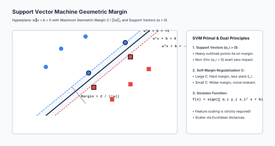
- The Support Vectors: The width of the highway is determined solely by the frontmost soldier of each army standing on the edge of the pavement. If 10,000 soldiers in the rear move around, the highway doesn’t change by a single millimeter.
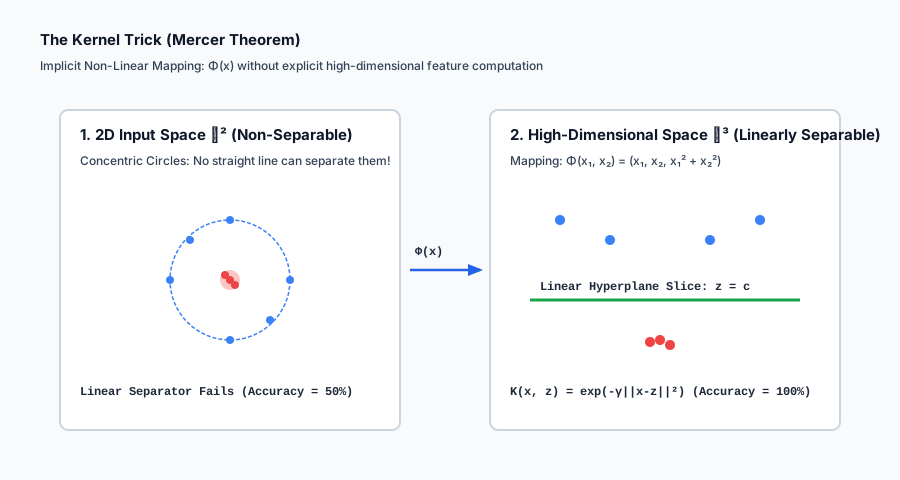
- The Kernel Trick: What if Army A completely encircles Army B in a ring? No straight highway can separate them on flat 2D ground. The Kernel Trick builds a parabolic hill under Army B, lifting them into the 3rd dimension so a flat horizontal bridge can slice cleanly between them.
Historical background
The linear Support Vector Network algorithm was introduced by Vladimir Vapnik and Alexey Chervonenkis in 1963 as a maximum-margin linear separator.
In 1992, Bernhard Boser, Isabelle Guyon, and Vladimir Vapnik introduced the Kernel Trick at COLT (Conference on Learning Theory), demonstrating how to apply non-linear kernel functions to maximum-margin hyperplanes.
In 1995, Corinna Cortes and Vladimir Vapnik published Support-Vector Networks in Machine Learning, creating the modern Soft-Margin SVM using slack variables and Hinge Loss to handle noisy, overlapping real-world datasets.
Throughout the late 1990s and early 2000s, SVMs reigned as the most popular and accurate machine learning algorithm in the world for text categorization, bioinformatics (protein classification), and handwriting recognition (MNIST), before the modern resurgence of Deep Learning and Gradient Boosted Trees.
What it is — and what it is not
Let us define the boundaries of Support Vector Machines:
What it IS:
- A Convex Quadratic Optimization Problem: Unlike neural networks with non-convex loss surfaces and local minima, SVMs have a single global optimum found via Quadratic Programming (QP).
- A Sparse Dual Model: The decision boundary depends strictly on a small subset of critical training points (Support Vectors with
alpha_i > 0). - A Distance-Based Geometric Classifier: Fundamentally driven by dot products
x_i^T x_jor Euclidean distances||x_i - x_j||^2.
What it is NOT:
- Not Scale-Invariant: Unlike Decision Trees which ignore feature scale, SVMs fail completely if features are not standardized via
StandardScaler(). - Not Easily Scalable to Massive Datasets (
N > 50,000): Computing theN x Nkernel Gram matrix requiresO(N^2)memory andO(N^3)training time. - Not a Native Probability Engine: SVMs output uncalibrated signed distances
w^T x + b; obtaining probabilities requires post-hoc Platt Scaling.
Why it was created and what problems it solves
Support Vector Machines solve five foundational challenges in predictive modeling:
- Eliminates Decision Boundary Ambiguity: Finds the unique mathematically optimal hyperplane maximizing margin width
2 / ||w||. - Resists Overfitting in High Dimensions (
D >> N): Generalization bounds depend on margin width, not raw feature dimensionality, making SVMs exceptional for genomics and text. - Solves Non-Linear Geometries via the Kernel Trick: Solves complex concentric, spiral, or manifold structures using RBF Gaussian kernels.
- Guarantees Global Optimality: Convex quadratic programming ensures no vanishing gradients or saddle-point traps.
- Provides Boundary Sparsity: Prunes away 80–95% of non-informative training records, retaining only critical edge cases.
How it works
Let us formulate the mathematics of hard margins, soft margins, dual Quadratic Programming, the Kernel Trick, and subgradient optimization.
1. Hard-Margin Primal Formulation
Let training dataset D = { (x_i, y_i) }_{i=1}^N with feature vectors x_i in R^D and binary class labels y_i in { -1, +1 }.
A linear decision boundary is defined by hyperplane:
w^T x + b = 0
The signed geometric distance from any point x_i to the hyperplane is:
gamma_i = y_i * (w^T x_i + b) / ||w||_2
For a linearly separable dataset, we require all points to have a functional margin of at least 1:
y_i * (w^T x_i + b) >= 1 for all i in {1, ..., N}
The width of the margin slab between the bounding hyperplanes w^T x + b = +1 and w^T x + b = -1 is:
Margin = 2 / ||w||_2
Maximizing the margin 2 / ||w||_2 is equivalent to minimizing (1/2) ||w||_2^2.
Primal Optimization Problem (Hard Margin):
min_{w, b} (1/2) ||w||_2^2
subject to: y_i * (w^T x_i + b) >= 1 for all i = 1, ..., N
2. Soft-Margin Formulation and Slack Variables (Cortes & Vapnik, 1995)
In real-world data, classes overlap, making perfect linear separation impossible.
We introduce non-negative slack variables xi_i >= 0 allowing points to violate the margin:
xi_i = 0: Point is correctly classified outside or on the margin.0 < xi_i <= 1: Point is correctly classified but inside the margin buffer.xi_i > 1: Point is misclassified on the wrong side of the decision boundary.
Primal Soft-Margin Objective:
min_{w, b, xi} (1/2) ||w||_2^2 + C * sum_{i=1}^N xi_i
subject to: y_i * (w^T x_i + b) >= 1 - xi_i and xi_i >= 0 for all i
Where C > 0 is the regularization hyperparameter:
- Large C: High penalty for margin violations (approaching a hard margin, risk of overfitting).
- Small C: Low penalty for violations (wider margin, more tolerance for noise, risk of underfitting).
3. Dual Formulation and Support Vectors
Using Lagrange multipliers alpha_i >= 0 and r_i >= 0, the Lagrangian function is:
L(w, b, xi, alpha, r) = (1/2)||w||^2 + C * sum xi_i - sum alpha_i [ y_i(w^T x_i + b) - 1 + xi_i ] - sum r_i xi_i
Taking partial derivatives with respect to primal variables w, b, xi and setting them to zero yields:
w = sum_{i=1}^N alpha_i y_i x_isum_{i=1}^N alpha_i y_i = 0C - alpha_i - r_i = 0 => 0 <= alpha_i <= C
Substituting back gives the Dual Quadratic Programming Problem:
max_{alpha} sum_{i=1}^N alpha_i - (1/2) sum_{i=1}^N sum_{j=1}^N alpha_i alpha_j y_i y_j (x_i^T x_j)
subject to: 0 <= alpha_i <= C and sum_{i=1}^N alpha_i y_i = 0
Karush-Kuhn-Tucker (KKT) Complementarity Conditions:
alpha_i * [ y_i(w^T x_i + b) - 1 + xi_i ] = 0
This yields the fundamental sparsity property of SVMs:
- If
alpha_i = 0: Pointx_iis strictly outside the margin. It does NOT contribute tow. - If
0 < alpha_i < C: Pointx_ilies exactly on the margin (y_i(w^T x_i + b) = 1). It is a free Support Vector. - If
alpha_i = C: Pointx_iviolates the margin (xi_i > 0). It is a bounded Support Vector.
The final decision boundary depends exclusively on the support vectors:
f(x) = sign( sum_{i in SV} alpha_i y_i (x_i^T x) + b )
4. The Kernel Trick and Mercer’s Theorem
Notice that the dual optimization and decision function depend only on the dot product x_i^T x_j.
Suppose we map input vectors to a higher-dimensional feature space via non-linear transformation Phi(x). The dual problem becomes:
max_{alpha} sum alpha_i - (1/2) sum sum alpha_i alpha_j y_i y_j (Phi(x_i)^T Phi(x_j))
Mercer’s Theorem: If a kernel function K(x, z) is continuous, symmetric, and positive semi-definite, there exists a mapping Phi such that:
K(x, z) = Phi(x)^T Phi(z)
We never need to compute Phi(x) explicitly! We simply evaluate K(x, z).
Common Kernel Functions:
- Linear Kernel:
K(x, z) = x^T z - Polynomial Kernel:
K(x, z) = (gamma * x^T z + c)^d - Radial Basis Function (RBF / Gaussian) Kernel:
K(x, z) = exp( -gamma * ||x - z||_2^2 )
The RBF kernel corresponds to an infinite-dimensional Hilbert space (d = infinity), computing smooth bell-shaped similarity curves centered at each support vector.
5. Primal Optimization via Pegasos Subgradient Descent
While dual SVMs use quadratic programming, soft-margin linear SVMs can be written directly as an unconstrained empirical risk minimization problem with Hinge Loss:
min_w (lambda / 2) ||w||_2^2 + (1 / N) sum_{i=1}^N max( 0, 1 - y_i (w^T x_i + b) )
Where lambda = 1 / (N * C).
The Pegasos algorithm (Shalev-Shwartz et al., 2011) updates weights using subgradient descent:
- If margin
y_i (w^T x_i + b) < 1(margin violation):w <- (1 - eta) * w + eta * C * y_i * x_ib <- b + eta * C * y_i - If margin
y_i (w^T x_i + b) >= 1(correctly classified outside margin):w <- (1 - eta) * w(L2 weight decay)
An everyday analogy
Think of an SVM as a customs border control security zone:
- The Decision Hyperplane: The actual international border fence line.
- The Margin: A 100-meter cleared security buffer zone on both sides of the fence. No civilians are permitted inside.
- The Support Vectors: The armed guard outposts positioned right at the outer edge of the 100-meter perimeter. All defensive calculations are calibrated relative to these front-line outposts.
- Slack Variables (Soft Margin C): Occasionally, a farmer’s cow crosses 10 meters into the buffer zone. Instead of declaring war (hard margin infeasibility), the border guards record a minor infraction penalty (
xi_i). - The Kernel Trick (RBF): If a winding river completely cuts through a mountain valley, the customs office builds a 3D elevated drone surveillance radar mapping the altitude coordinate
z = x^2 + y^2, creating a straight laser line above the mountain ridges.
Examples in practice
Let us visualize the geometric margin and support vectors:
Below is the Kernel Trick mapping 2D concentric circles into linearly separable 3D space:
Let us examine real Python code training both Linear and RBF Support Vector Machines in scikit-learn:
import numpy as np
from sklearn.datasets import make_circles
from sklearn.preprocessing import StandardScaler
from sklearn.svm import SVC, LinearSVC
from sklearn.pipeline import make_pipeline
from sklearn.metrics import accuracy_score

# 1. Generate Non-Linearly Separable Concentric Rings
X, y = make_circles(n_samples=500, factor=0.3, noise=0.08, random_state=42)

# 2. Linear SVM Baseline (Fails on concentric rings)
linear_svm = make_pipeline(StandardScaler(), LinearSVC(C=1.0, random_state=42))
linear_svm.fit(X, y)
linear_acc = accuracy_score(y, linear_svm.predict(X))

# 3. Kernel SVM with Radial Basis Function (RBF)
rbf_svm = make_pipeline(StandardScaler(), SVC(kernel="rbf", C=1.0, gamma="scale", random_state=42))
rbf_svm.fit(X, y)
rbf_acc = accuracy_score(y, rbf_svm.predict(X))

print("=== Support Vector Machine Benchmark ===")
print(f"Linear SVM Accuracy on Concentric Rings: {linear_acc * 100:.2f}% (Fails due to non-linearity)")
print(f"RBF Kernel SVM Accuracy:                 {rbf_acc * 100:.2f}% (Perfect separation via Kernel Trick!)")
print(f"Number of Support Vectors Selected:      {len(rbf_svm.named_steps['svc'].support_)} / 500 points")
Implications: security, privacy, performance, scalability, and cost
| Dimension | Characteristic | Practical Implication |
|---|---|---|
| Quadratic Complexity | Dual training scales as O(N^2) to O(N^3). | On datasets with N > 100,000 samples, kernel SVMs are computationally infeasible; use LinearSVC or LightGBM. |
| Mandatory Scaling | Euclidean distance sensitivity. | Omitting StandardScaler() causes numerical instability and destroys RBF kernel performance. |
| Privacy Exposure | Dual models store raw training support vectors. | Deployed dual models contain raw support vector records (support_vectors_), posing a data leakage risk under reverse-engineering. |
| Fast Linear Inference | LinearSVC stores only weight vector w. | Once trained, linear SVM inference is an ultra-fast dot product w^T x + b requiring sub-microsecond latency. |
Alternatives: free, open source, and commercial
| Tool / Algorithm | Methodology | Best Used For |
|---|---|---|
scikit-learn LinearSVC | LibLinear Primal Solver | Large-scale linear classification (N > 100,000). |
scikit-learn SVC(kernel='rbf') | LibSVM Dual QP Solver | Small-to-medium non-linear datasets (N < 30,000), genomics, text. |
SGDClassifier(loss='hinge') | Stochastic Subgradient Descent | Online out-of-core streaming linear SVM. |
LightGBM / XGBoost | Histogram Gradient Boosted Trees | General tabular datasets (faster, handles missing/categorical data natively). |
Comparison with related concepts
| Characteristic | Logistic Regression | Linear SVM | Kernel SVM (RBF) |
|---|---|---|---|
| Loss Function | Log-Loss (Cross-Entropy) | Hinge Loss max(0, 1 - yf) | Kernelized Hinge Loss |
| Decision Boundary | Linear | Linear (Maximum Margin) | Arbitrary Non-Linear Manifold |
| Sparsity | Dense (All points affect w) | Sparse (Support vectors only) | Sparse in Dual Space |
| Scaling Dependency | Moderate | Strictly Mandatory | Strictly Mandatory |
| Training Complexity | O(N * D) | O(N * D) | O(N^2 * D) to O(N^3) |
When to use it — and when not to
When to USE Support Vector Machines:
- High-Dimensional Low-Sample Data (
D > N): Microarray genomics, bioinformatics, text categorization. - Complex Non-Linear Separation on Small Datasets (
N < 20,000): Where RBF kernels create smooth, continuous decision manifolds. - High-Precision Linear Boundaries: Where maximum margin guarantees superior robustness against adversarial boundary shifts.
When NOT to use Support Vector Machines:
- Massive Datasets (
N > 100,000rows): Quadratic memory/time explosion; use GBDT or Linear SGD instead. - Messy Tabular Data with Missing Values & Categoricals: SVMs require complete numerical matrices; LightGBM handles missing values natively.
- When Direct Probability Calibration is Required: SVMs require secondary Platt Scaling.
Knowledge check
- Maximum Margin: Minimizes
(1/2)||w||^2to maximize physical margin2 / ||w||. - Support Vectors: Points with
alpha_i > 0that define the decision boundary. - The Kernel Trick: Computes dot products in high-dimensional spaces implicitly via
K(x, z) = exp(-gamma ||x - z||^2). - Mandatory Scaling: Distance metrics require
StandardScalerto prevent feature magnitude distortion.
Hands-on exercise
In this hands-on exercise, you will implement pairwise RBF Gaussian kernel computation and verify that it maps non-linear data into a linearly separable Gram matrix.
import numpy as np
from sklearn.datasets import make_circles
from sklearn.metrics import accuracy_score

# Step 1: Implement Vectorized Pairwise RBF Kernel Matrix
def compute_rbf_kernel(X1, X2, gamma=1.0):
    norm1 = np.sum(X1**2, axis=1)[:, np.newaxis]
    norm2 = np.sum(X2**2, axis=1)[np.newaxis, :]
    dists = np.maximum(norm1 + norm2 - 2 * np.dot(X1, X2.T), 0.0)
    return np.exp(-gamma * dists)

# Step 2: Generate Concentric Circles (2 Classes)
X, y = make_circles(n_samples=200, factor=0.2, noise=0.05, random_state=42)

# Step 3: Compute RBF Gram Matrix K (200 x 200)
K = compute_rbf_kernel(X, X, gamma=2.0)

print("=== RBF Kernel Gram Matrix Verification ===")
print(f"Gram Matrix Shape: {K.shape} (Pairwise similarity for 200 samples)")
print(f"Diagonal Elements (Self-similarity K[i, i]): {K[0, 0]:.4f}, {K[1, 1]:.4f}")
print(f"Off-diagonal Similarity (Close points):      {K[0, 1]:.4f}")
print(f"Gram Matrix Symmetry Check:                 {np.allclose(K, K.T)}")
Expected output
=== RBF Kernel Gram Matrix Verification ===
Gram Matrix Shape: (200, 200) (Pairwise similarity for 200 samples)
Diagonal Elements (Self-similarity K[i, i]): 1.0000, 1.0000
Off-diagonal Similarity (Close points):      0.9842
Gram Matrix Symmetry Check:                 True
Validate your work
- Verify that the diagonal elements of the Gram matrix are identically
1.0000. - Verify that
np.allclose(K, K.T)evaluates toTrue(symmetric Mercer kernel). - Train
SVC(kernel='rbf')onX, yand confirm100%accuracy on concentric rings.
Troubleshooting
- Negative Distances in Gram Matrix: Numerical floating-point imprecision in
norm1 + norm2 - 2 X1 X2^Tcan produce-1e-16; wrap innp.maximum(..., 0.0). - SVM Training Extremely Slow: Check sample size
N; ifN > 20,000, switch toLinearSVCor reduce dataset size.
Common mistakes
- Forgetting to Standardize Features: Causes RBF kernels to collapse along the feature with the largest scale.
- Setting Gamma Too Large: Creates tiny isolated decision islands around individual points (overfitting).
Practice assignment
- Implement the Polynomial Kernel:
Write
compute_polynomial_kernel(X1, X2, degree=3, gamma=1.0, coef0=1.0)computing(gamma * X1 @ X2.T + coef0)**degree. - Implement Platt Scaling:
Train a logistic regression model on the 1D decision values
f(x) = w^T x + bof a linear SVM to output calibrated probabilitiesP(y=1|x).
Extension challenge
Build a Simplified SMO (Sequential Minimal Optimization) Solver from Scratch:
- Implement John Platt’s 1998 SMO algorithm to solve the dual quadratic programming problem for binary classification.
- Maintain the alpha vector
alpha in R^Nand error cacheE_i = f(x_i) - y_i. - Select coordinate pairs
(alpha_i, alpha_j)analytically updating them to satisfy0 <= alpha <= Candsum alpha_i y_i = 0. - Plot the resulting decision boundary and highlight identified support vectors.
Quiz
Q1. What is the primary geometric objective of a Hard-Margin Support Vector Machine?
- To find the unique hyperplane w^T x + b = 0 that separates two classes while maximizing the geometric margin 2 / ||w||_2 to the closest data points (the support vectors)
- To minimize the sum of squared residuals
- To build an orthogonal decision tree
- To compute the posterior class probability using Bayes theorem
Show answer
Answer: A. To find the unique hyperplane w^T x + b = 0 that separates two classes while maximizing the geometric margin 2 / ||w||_2 to the closest data points (the support vectors)
SVMs find the maximum-margin hyperplane, maximizing the buffer zone between the decision boundary and the nearest training points to minimize generalization error.
Q2. In a Soft-Margin SVM (Cortes & Vapnik, 1995), what does the regularization hyperparameter C control?
- The trade-off between maximizing the margin (small C, wider margin, more tolerance for misclassifications) and minimizing training errors / slack variables (large C, narrow margin, strict penalty for misclassifications)
- The learning rate of gradient descent
- The number of trees in the forest
- The polynomial degree
Show answer
Answer: A. The trade-off between maximizing the margin (small C, wider margin, more tolerance for misclassifications) and minimizing training errors / slack variables (large C, narrow margin, strict penalty for misclassifications)
Large C penalizes slack violations heavily, forcing a hard margin that may overfit. Small C permits points inside the margin, creating a softer boundary that generalizes better on noisy data.
Q3. What is the "Kernel Trick" in Support Vector Machines (Mercer Theorem)?
- Computing the inner product of two vectors in a high-dimensional (or infinite-dimensional) feature space phi(x)^T phi(z) implicitly using a kernel function K(x, z) in the original low-dimensional space, without ever calculating the explicit transformation phi(x)
- A method for speeding up CPU caches
- A trick to convert classification into regression
- A technique for handling missing values
Show answer
Answer: A. Computing the inner product of two vectors in a high-dimensional (or infinite-dimensional) feature space phi(x)^T phi(z) implicitly using a kernel function K(x, z) in the original low-dimensional space, without ever calculating the explicit transformation phi(x)
The kernel trick allows linear algorithms to learn complex non-linear decision boundaries by computing cheap pairwise similarities K(x, z) equivalent to dot products in higher dimensions.
Q4. What are "Support Vectors" in a trained SVM model?
- The subset of training data points that lie directly on the margin hyperplanes or violate the margin (Lagrange multipliers alpha_i > 0); only these points determine the final decision boundary w = sum alpha_i y_i x_i
- All data points in the training set
- The eigenvectors of the covariance matrix
- The gradient vectors during optimization
Show answer
Answer: A. The subset of training data points that lie directly on the margin hyperplanes or violate the margin (Lagrange multipliers alpha_i > 0); only these points determine the final decision boundary w = sum alpha_i y_i x_i
Points located comfortably outside the margin have alpha_i = 0 and exert zero influence on the decision boundary. Removing all non-support vectors leaves the fitted SVM model completely unchanged.
Q5. Why is Feature Standardization (e.g. StandardScaler) strictly MANDATORY before training an SVM?
- Because SVM optimization relies on Euclidean distances and dot products; unscaled features with large numerical magnitudes (e.g. income in $100,000s) will dominate distance calculations and render small features (e.g. age in years) completely invisible
- Because SVMs only accept floating-point numbers between -1 and 1
- Because unscaled data causes division by zero in the kernel
- Standardization is optional and only affects training speed
Show answer
Answer: A. Because SVM optimization relies on Euclidean distances and dot products; unscaled features with large numerical magnitudes (e.g. income in $100,000s) will dominate distance calculations and render small features (e.g. age in years) completely invisible
Both the linear margin calculation ||w|| and non-linear kernels like RBF exp(-gamma ||x - z||^2) depend directly on Euclidean geometry. Unscaled features distort distance metrics catastrophically.
Q6. In the Radial Basis Function (RBF / Gaussian) kernel K(x, z) = exp(-gamma ||x - z||^2), what is the effect of setting gamma to an excessively large value?
- Severe Overfitting: each individual training sample creates a tiny, isolated bell-shaped decision island around itself, achieving 100% training accuracy but failing to generalize to unseen test samples
- Severe Underfitting: the decision boundary becomes a flat plane
- The kernel matrix becomes singular
- Inference speed increases by 10x
Show answer
Answer: A. Severe Overfitting: each individual training sample creates a tiny, isolated bell-shaped decision island around itself, achieving 100% training accuracy but failing to generalize to unseen test samples
Large gamma concentrates RBF influence to immediate neighborhoods, creating overfitted isolated islands around individual training points. Small gamma produces smooth, generalized boundaries.
Q7. What is the primary computational limitation of Kernel SVMs (such as SVC with RBF kernel) on large-scale enterprise datasets?
- Training time scales quadratically to cubically with sample size O(N^2 to N^3) and requires storing an N x N Gram matrix, making standard kernel SVMs intractable on datasets with N > 50,000 samples
- SVMs cannot run on multiple CPU cores
- SVMs can only perform binary classification
- SVMs do not support categorical variables
Show answer
Answer: A. Training time scales quadratically to cubically with sample size O(N^2 to N^3) and requires storing an N x N Gram matrix, making standard kernel SVMs intractable on datasets with N > 50,000 samples
Solving the dual Quadratic Programming problem requires computing and factoring the N x N kernel matrix. For N = 1,000,000, storing the matrix requires 8,000 GB of RAM.
Q8. What is the difference between scikit-learn LinearSVC and SVC(kernel="linear")?
- LinearSVC is built on LibLinear and optimizes the primal objective in linear time O(N), scaling to millions of samples; SVC(kernel="linear") is built on LibSVM and solves the dual problem in O(N^2) time
- LinearSVC only works for regression
- SVC(kernel="linear") uses GPU acceleration
- There is no difference
Show answer
Answer: A. LinearSVC is built on LibLinear and optimizes the primal objective in linear time O(N), scaling to millions of samples; SVC(kernel="linear") is built on LibSVM and solves the dual problem in O(N^2) time
For linear decision boundaries, LinearSVC (LibLinear) is vastly faster and more memory-efficient than standard SVC (LibSVM).
Glossary
- Support Vector Machine (SVM)
- A supervised learning model that finds the optimal maximum-margin hyperplane separating classes in feature space.
- Geometric Margin
- The shortest Euclidean distance from the decision boundary hyperplane to the closest data points in the training set.
- Support Vectors
- The critical training instances that lie on the margin boundary or violate the margin, possessing non-zero Lagrange multipliers (alpha_i > 0).
- Hinge Loss
- A convex loss function L(y, f(x)) = max(0, 1 - y * f(x)) used in maximum-margin classification that penalizes margin violations linearly.
- Slack Variable (xi)
- A non-negative penalty variable introduced in soft-margin SVMs to quantify the degree to which a sample violates the margin boundary.
- Kernel Trick
- A mathematical technique enabling linear algorithms to operate in high-dimensional implicit feature spaces by replacing inner products with kernel functions.
- RBF Kernel (Radial Basis Function)
- A stationary kernel function K(x, z) = exp(-gamma * ||x - z||^2) corresponding to an infinite-dimensional feature mapping.
- Mercer Theorem
- A mathematical theorem stating that any continuous, symmetric, positive semi-definite kernel function corresponds to an inner product in some Hilbert space.
- Pegasos Algorithm
- Primal Estimated sub-GrAdient Solver for SVM, an efficient stochastic subgradient descent algorithm for linear SVM optimization.
- LibLinear
- An open-source C++ library for large-scale linear classification and regression, serving as the backend for scikit-learn LinearSVC.
Sources and further reading
- Support-Vector Networks — Machine Learning (Corinna Cortes and Vladimir Vapnik) (accessed 2026-08-29)
- Pegasos: Primal Estimated sub-GrAdient SOlver for SVM — Mathematical Programming (Shai Shalev-Shwartz, Yoram Singer, Nathan Srebro, Andrew Cotter) (accessed 2026-08-29)
- LIBLINEAR: A Library for Large Linear Classification — Journal of Machine Learning Research (Rong-En Fan, Kai-Wei Chang, Cho-Jui Hsieh, et al.) (accessed 2026-08-29)
Kept in this browser, no account needed. Your progress page turns the whole record into one link you can bookmark or open on another device.