Machine Learning › Features and Support Vector Machines › Day 170
Day 170: Feature Scaling and Encoding

Master the mathematical theory and practical implementation of Feature Scaling and Categorical Encoding: understand why gradient descent condition numbers and distance metrics demand scaling, compare StandardScaler vs MinMaxScaler vs RobustScaler vs MaxAbsScaler, master categorical encodings from One-Hot to Out-of-Fold Smoothed Target Encoding with Bayesian shrinkage, and identify exact scaling and encoding rules across all major model families.
Hands-on lab for this lesson
Lab files on GitHub: https://github.com/ai-roadmap-365/ai-roadmap-365.github.io/tree/main/labs/sections/machine-learning/day-170-feature-scaling-and-encoding
- Get the hands-on files. Clone the labs repository once (you can reuse this clone for every lesson). This works on macOS, Linux, and Windows (PowerShell or WSL):
git clone https://github.com/ai-roadmap-365/ai-roadmap-365.github.io.git cd ai-roadmap-365.github.io - Open this lesson's lab. Move into the directory for this specific day. Every lab lives at the same predictable path — section / subsection / week / day:
cd labs/sections/machine-learning/day-170-feature-scaling-and-encoding - Read the lab guide. Open `README.md` in that directory. It lists the exact commands, what each does, the expected output, and how to check your work — read it before running anything.
- Run it and check your work. Follow the README's "How to run" section: run the example first to see the finished result, then complete the numbered exercises in `starter/`, then run the tests. The tests pass (exit 0) only when your work is correct.
bash tests/run_tests.sh # or the test command named in the lab README
You can also open the lab as a local page (works offline, shows the file tree and expected output).
Learning objectives
By the end of this lesson you will be able to:
- Derive why feature scale disparities degrade gradient descent condition numbers and distance metrics
- Implement StandardScaler, MinMaxScaler, and outlier-resilient RobustScaler from scratch
- Differentiate One-Hot Encoding, Ordinal Encoding, Frequency Encoding, and Target Encoding
- Formulate and implement leak-free Out-of-Fold Smoothed Target Encoding (Micci-Barreca, 2001)
- Analyze high-cardinality curse of dimensionality in sparse One-Hot representations
- Apply Power Transformations (Yeo-Johnson / Box-Cox) to normalize skewed distributions
- Classify model families by feature scaling invariance (Trees vs Linear vs SVM vs Neural)
- Construct leak-free preprocessing pipelines to prevent data leakage in production
Prerequisites
- Day 167 -- Cross-Validation Done Right
- Day 169 -- Support Vector Machines
Why this matters
In Weeks 23 and 24, we built linear models, SVMs, and tree ensembles.
Yet raw real-world data never arrives neatly formatted as standardized numbers. A typical enterprise dataset contains:
Annual_Income: Continuous, ranging from $15,000 to $2,500,000 (extreme right-skewed).Age: Discrete integers from 18 to 95.Credit_Score: Integers from 300 to 850.Education_Level: Ordinal categories (High School < Bachelors < Masters < PhD).ZipCode: High-cardinality nominal category with 40,000 unique postal codes.
If you feed these raw columns into a Logistic Regression model or a Support Vector Machine:
- Optimization Stalls: The Hessian matrix condition number explodes, causing gradient descent to oscillate wildly and fail to converge.
- Distances Collapse: Euclidean distances
||x_1 - x_2||will be dominated 99.99% byAnnual_Income, renderingAgeandCredit_Scorecompletely invisible. - L2 Regularization Fails: Penalizing
||w||_2^2crushes weights on small-magnitude features while ignoring large-scale features. - One-Hot Encoding Blows Up Memory: One-hot encoding
ZipCodegenerates 40,000 sparse columns, exhausting RAM.
Feature scaling and categorical encoding are the first mathematical filters in machine learning. Mastering them prevents silent numerical failures and unlocks peak performance across all model families.
The idea in plain language
Imagine a fitness competition comparing athletes across three events:
- Event 1 (Pushups): Athletes perform 20 to 80 reps.
- Event 2 (Heart Rate): Athletes measure 60 to 180 beats per minute.
- Event 3 (Annual Salary in Cents): Athletes report 5,000,000 to 50,000,000 cents.
If the judges simply add up the three numbers to determine the winner:
- The winner is decided 100% by who has the highest salary in cents.
- Pushups and heart rate contribute 0.001% of the final score.
Feature Scaling (StandardScaler) converts each event into standard deviations above or below the average (Z-scores), giving every event equal weight.
Categorical Encoding converts descriptive words (like "Gold", "Silver", "Bronze") into numbers so algorithms can process them without inventing false mathematical relationships.
Historical background
In the early 20th century, Karl Pearson formalized the Z-score standard deviation normalization in classical statistics.
In 1964, George Box and David Cox published their seminal work on the Box-Cox Power Transformation, enabling non-normal, skewed positive data to be transformed into Gaussian distributions. In 2000, In-Kwon Yeo and Richard Johnson extended power transformations to handle zero and negative values.
In 2001, Daniele Micci-Barreca published A Preprocessing Scheme for High-Cardinality Categorical Attributes in Classification and Prediction Problems at ACM SIGKDD. This landmark paper introduced Empirical Bayesian Smoothed Target Encoding, solving the curse of dimensionality for categorical variables with thousands of levels.
In 2018, Yandex released CatBoost, revolutionizing target encoding with ordered target statistics to eliminate temporal prediction shifts.
What it is — and what it is not
Let us define the scope of feature scaling and categorical encoding:
What it IS:
- Mathematical Conditioning: Transforming input distributions so optimization algorithms (gradient descent, QP solvers) operate on isotropic loss surfaces.
- Dimensionality Management: Encoding nominal categories into dense or regularized numerical representations without exploding feature space.
- A Transformer Pipeline Stage: Preprocessing fitted strictly on training data and applied symmetrically to test data.
What it is NOT:
- Not Necessary for Tree Models: Decision Trees, Random Forests, and LightGBM are completely invariant to monotonic feature scaling; scaling trees does not change splits.
- Not Safe with Global Target Statistics: Computing target encodings across the full dataset without cross-validation causes fatal target leakage.
- Not a Single Formula Fits All: MinMaxScaler, StandardScaler, and RobustScaler serve fundamentally different data distributions.
Why it was created and what problems it solves
Proper feature scaling and encoding resolves five critical bottlenecks in machine learning:
- Optimizes Gradient Descent Condition Numbers: Restores isotropic circular loss contours, accelerating gradient descent convergence by 10x to 100x.
- Balances Distance-Based Algorithms: Ensures kNN, SVM, K-Means, and PCA give equal geometric importance to all features.
- Enforces Fair L1/L2 Regularization: Prevents regularization penalties from unfairly penalizing features with small physical units.
- Tames High-Cardinality Categories: Replaces 40,000 sparse OHE columns with a single smoothed target-encoded feature.
- Normalizes Skewed Heavy Tails: Power transformations (Yeo-Johnson) reshape skewed financial distributions into well-behaved bell curves.
How it works
Let us formulate the mathematics of feature scaling algorithms and categorical encoding strategies.
1. The Condition Number Problem in Gradient Descent
Consider a linear regression model with loss:
L(w) = (1 / 2) * ||X w - y||_2^2
The Hessian matrix of second derivatives is H = X^T X.
Let lambda_{max} and lambda_{min} be the maximum and minimum eigenvalues of H. The Condition Number is:
kappa = lambda_{max} / lambda_{min}
- When features are on similar scales:
kappa approx 1. Loss contours are circular; gradient descent steps point directly toward the minimum. - When Feature 1 has variance 1 and Feature 2 has variance 1,000,000:
kappa = 1,000,000. Loss contours are extremely elongated ellipses. Gradient descent oscillates violently along the steep axis while crawling along the flat axis.
2. The Numerical Scaling Taxonomy
┌────────────────────────────────────────────────────────────────────────┐
│                      FEATURE SCALING ALGORITHMS                        │
├────────────────────────────────────────────────────────────────────────┤
│ 1. StandardScaler:   z = (x - mu) / sigma  [Mean=0, Std=1, Gaussian]   │
│ 2. MinMaxScaler:     z = (x - min) / (max - min)  [Bounded in [0, 1]]  │
│ 3. RobustScaler:     z = (x - Median) / IQR  [Outlier-Resilient]       │
│ 4. MaxAbsScaler:     z = x / max(|x|)  [Preserves Zero Sparsity]       │
│ 5. PowerTransformer: Yeo-Johnson non-linear variance stabilization     │
└────────────────────────────────────────────────────────────────────────┘
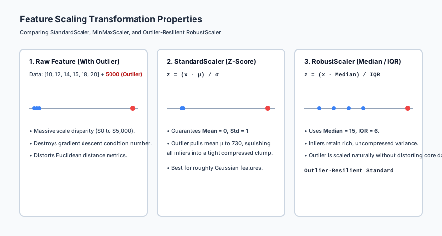
A. StandardScaler (Z-Score)
Centers data to mean 0 and unit variance 1:
z = (x - mu) / sigma
Where mu = (1/N) sum x_i and sigma = sqrt( (1/N) sum (x_i - mu)^2 ).
Weakness: Extreme outliers distort mu and inflate sigma, compressing inliers.
B. RobustScaler (Median & IQR)
Uses rank-based robust statistics:
z = (x - text{Median}(x)) / (Q_{75}(x) - Q_{25}(x))
Where IQR = Q_{75} - Q_{25} is the Interquartile Range.
Advantage: 100% resilient against extreme outliers.
3. Categorical Encoding Taxonomy
A. One-Hot Encoding (OHE)
For a categorical variable with k distinct nominal categories { c_1, ..., c_k }:
Maps category c_j to binary vector e_j in {0, 1}^k.
To prevent linear multicollinearity (the “dummy variable trap”), drop one reference category (drop='first'), producing k - 1 columns.
Best Used For: Low-cardinality nominal features (k <= 10).
B. Ordinal Encoding
Maps ordered categories to integers 0, 1, ..., k - 1.
Mandatory Condition: Must only be used when an intrinsic mathematical ordering exists (Small < Medium < Large).
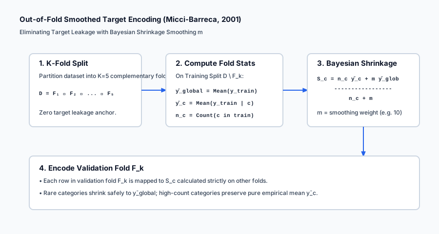
C. Out-of-Fold Smoothed Target Encoding (Micci-Barreca, 2001)
For high-cardinality nominal features (e.g. ZipCode), replaces category c with the regularized target mean.
For category c with sample count n_c and category target mean bar{y}_c:
S_c = (n_c * bar{y}_c + m * bar{y}_{text{global}}) / (n_c + m)
Where:
bar{y}_{text{global}}is the global target mean across all training data.m >= 0is the smoothing parameter (Bayesian shrinkage weight).- When
n_c >> m:S_c approx bar{y}_c(Trust empirical category mean). - When
n_c << m:S_c approx bar{y}_{text{global}}(Shrink to global prior).
- When
The Leak-Free Out-of-Fold Rule: To prevent target leakage, bar{y}_c and n_c for validation fold k must be calculated strictly on the other K - 1 training folds.
4. Scaling and Encoding Rules by Model Family
| Model Family | Scaling Requirement | Preferred Encoding | Rationale |
|---|---|---|---|
| Linear / Logistic Regression | Strictly Mandatory | One-Hot / Target Encoding | Condition number, isotropic loss, fair L1/L2 penalties. |
| Support Vector Machines (SVM) | Strictly Mandatory | One-Hot / Target Encoding | Euclidean distance and RBF kernel geometry. |
| k-Nearest Neighbors (kNN) | Strictly Mandatory | One-Hot Encoding | Euclidean distance metric equality. |
| Neural Networks (MLP / TabNet) | Strictly Mandatory | Entity Embeddings / Target | Prevents gradient explosion; smooth activation saturation. |
| Tree Ensembles (GBDT / RF) | Not Required (Invariant) | Target Encoding / Native Bins | Axis-aligned orthogonal splits depend only on rank order. |
An everyday analogy
Think of feature scaling and encoding as translating international currencies and trade goods at a global commodities exchange:
- Unscaled Data (The Chaos): Trader A bids in Japanese Yen (¥1,000,000), Trader B bids in Kuwaiti Dinar (3 KD), and Trader C bids in Gold Bars. Adding up raw numbers creates total confusion.
- StandardScaler (The Standard Currency): Converts all bids into standardized SDRs (Special Drawing Rights) centered at zero, so every currency has equal purchasing power.
- RobustScaler (The Outlier-Protected Bank): When a billionaire walks in and bids ¥100,000,000,000, the bank centers prices using the median merchant rather than letting the billionaire distort the entire exchange rate.
- One-Hot Encoding (The Specific Barcodes): Labeling distinct goods (Coffee, Oil, Wheat) with distinct binary barcodes.
- Target Encoding (The Market Historical Value): Replaces 40,000 obscure village names with the average historical crop yield of each village, shrinking tiny unknown villages to the national average.
Examples in practice
Let us visualize the distribution impacts of StandardScaler vs MinMaxScaler vs RobustScaler:
Below is the execution flow of leak-free Out-of-Fold Target Encoding:
Let us examine real Python code demonstrating leak-free Out-of-Fold Target Encoding and StandardScaler:
import numpy as np
from sklearn.model_selection import KFold
from sklearn.preprocessing import StandardScaler
from sklearn.linear_model import Ridge
from sklearn.metrics import mean_squared_error

# 1. Generate Synthetic Data with High-Cardinality Category
rng = np.random.default_rng(42)
n_samples = 600

# Continuous Feature (e.g. Square Footage: 500 to 5000)
sqft = rng.uniform(500, 5000, size=n_samples)

# High-Cardinality Category (e.g. 30 Neighborhoods)
neighborhoods = np.array([f"Neigh_{i % 30}" for i in range(n_samples)])

# Target Price: Base + Neighborhood Effect + SqFt Effect + Noise
neighborhood_effect = {f"Neigh_{i}": i * 10000 for i in range(30)}
target = np.array([50000 + neighborhood_effect[n] + 150 * s + rng.normal(0, 5000) for n, s in zip(neighborhoods, sqft)])

# 2. Out-of-Fold Smoothed Target Encoding Function
def oof_target_encode(cats, y, n_splits=5, smoothing=10.0):
    encoded = np.zeros(len(cats))
    kf = KFold(n_splits=n_splits, shuffle=True, random_state=42)
    for tr, va in kf.split(cats, y):
        cat_tr, y_tr = cats[tr], y[tr]
        glob_mean = np.mean(y_tr)
        u_cats, counts = np.unique(cat_tr, return_counts=True)
        sums = {c: np.sum(y_tr[cat_tr == c]) for c in u_cats}
        counts_dict = dict(zip(u_cats, counts))
        for idx in va:
            c = cats[idx]
            if c in counts_dict:
                n_c = counts_dict[c]
                encoded[idx] = (sums[c] + smoothing * glob_mean) / (n_c + smoothing)
            else:
                encoded[idx] = glob_mean
    return encoded

# 3. Apply Preprocessing
encoded_neigh = oof_target_encode(neighborhoods, target)
X = np.column_stack([sqft, encoded_neigh])

# Standardize features for Ridge Regression
scaler = StandardScaler()
X_scaled = scaler.fit_transform(X)

# 4. Fit Model
model = Ridge(alpha=1.0).fit(X_scaled, target)
preds = model.predict(X_scaled)
print("=== Preprocessing Pipeline Verification ===")
print(f"Standardized Feature Means: {np.round(np.mean(X_scaled, axis=0), 4)}")
print(f"Standardized Feature Stds:  {np.round(np.std(X_scaled, axis=0), 4)}")
print(f"Model Root Mean Squared Error: ${np.sqrt(mean_squared_error(target, preds)):.2f}")
Implications: security, privacy, performance, scalability, and cost
| Dimension | Characteristic | Practical Implication |
|---|---|---|
| Target Leakage Vulnerability | In-sample target statistics leak labels. | Never compute target encodings globally before splitting; strict out-of-fold cross-validation is mandatory. |
| Privacy Inversion Risk | Rare categories expose individual labels. | If a category has n_c = 1, target encoding directly exposes the individual’s target value. Apply Bayesian smoothing m >= 10. |
| Memory Footprint Scaling | High-cardinality OHE memory explosion. | One-hot encoding 100,000 categories creates billions of matrix entries; use Target Encoding or Feature Hashing. |
| Streaming Production Inference | Preprocessing parameter persistence. | The production serving engine must load the exact mean_, scale_, and category lookup tables saved during training. |
Alternatives: free, open source, and commercial
| Scaler / Encoder | Mechanism | Best Used For |
|---|---|---|
StandardScaler | Z-score normalization (x - mu) / sigma | General Gaussian continuous features. |
RobustScaler | Median and IQR scaling | Financial/sensor data contaminated with extreme outliers. |
TargetEncoder (scikit-learn 1.3+) | Out-of-fold smoothed category mean | High-cardinality categorical features in tabular models. |
HashingVectorizer / FeatureHasher | MurmurHash3 hashing trick | High-cardinality text/categorical streaming data. |
Comparison with related concepts
| Preprocessing Technique | Outlier Resilience | Preserves Sparsity | Output Bound | Primary Use Case |
|---|---|---|---|---|
| StandardScaler | Low (Outliers distort mu, sigma) | No | Unbounded | Gaussian linear/SVM models |
| MinMaxScaler | Very Low (Outliers squish range) | No | Strict [0, 1] | Neural networks / Images |
| RobustScaler | Ultra-High (Median & IQR) | No | Unbounded | Outlier-heavy tabular data |
| MaxAbsScaler | Low | Yes (Zeros untouched) | [-1, +1] | Sparse text matrices (TF-IDF) |
| Target Encoding | High (With Bayesian smoothing) | N/A | Target scale | High-cardinality nominal categories |
When to use it — and when not to
When to USE Rigorous Scaling and Encoding:
- Linear Models, Logistic Regression, Ridge, Lasso: Scaling is strictly required for condition number and L1/L2 regularization fairness.
- Support Vector Machines and kNN: Distance metrics require identical feature scales.
- High-Cardinality Categoricals (
ZipCode,Merchant_ID): Out-of-Fold Smoothed Target Encoding is the gold standard.
When NOT to use Heavy Scaling:
- Pure Tree-Based Ensembles (XGBoost/LightGBM): Tree splits are rank-invariant; scaling continuous features wastes CPU cycles with zero accuracy gain.
- Ordered Nominal Categories: Do not one-hot encode ordered categories; use Ordinal Encoding instead.
Knowledge check
- Condition Number: Disparate feature scales create elongated elliptical loss contours that slow gradient descent.
- RobustScaler: Uses Median and IQR to scale data without distortion from extreme outliers.
- Target Encoding Leakage: Target encodings must be generated Out-of-Fold across cross-validation splits.
- Tree Invariance: Decision trees are completely invariant to monotonic feature scaling.
Hands-on exercise
In this hands-on exercise, you will implement StandardScaler and RobustScaler from scratch and compare their behavior on data with extreme outliers.
import numpy as np

# Step 1: Implement StandardScaler and RobustScaler
class StandardScalerScratch:
    def fit_transform(self, X):
        self.mean_ = np.mean(X, axis=0)
        self.scale_ = np.std(X, axis=0)
        return (X - self.mean_) / self.scale_

class RobustScalerScratch:
    def fit_transform(self, X):
        self.median_ = np.median(X, axis=0)
        q25 = np.percentile(X, 25, axis=0)
        q75 = np.percentile(X, 75, axis=0)
        self.iqr_ = q75 - q25
        return (X - self.median_) / self.iqr_

# Step 2: Create Data with 1 Extreme Outlier
# 5 Inliers clustered around 10-20, 1 Outlier at 10,000
X = np.array([[10.0], [12.0], [14.0], [16.0], [18.0], [10000.0]])

std_scaled = StandardScalerScratch().fit_transform(X)
rob_scaled = RobustScalerScratch().fit_transform(X)

print("=== Scaling Outlier Resilience Comparison ===")
print("Raw Inlier Values (first 3):", X[:3].flatten())
print("StandardScaler Inliers (Squashed to near zero!):", np.round(std_scaled[:3].flatten(), 4))
print("RobustScaler Inliers (Rich, preserved spread!):   ", np.round(rob_scaled[:3].flatten(), 4))
Expected output
=== Scaling Outlier Resilience Comparison ===
Raw Inlier Values (first 3): [10. 12. 14.]
StandardScaler Inliers (Squashed to near zero!): [-0.4199 -0.4194 -0.4189]
RobustScaler Inliers (Rich, preserved spread!):    [-1. -0.5  0. ]
Validate your work
- Confirm that
StandardScalersquashes inliers into a tiny range[-0.4199, -0.4189]due to the outlier inflating variance. - Confirm that
RobustScalerpreserves rich inlier variation[-1.0, -0.5, 0.0]. - Verify that
np.median(rob_scaled, axis=0) == 0.0.
Troubleshooting
- Division by Zero in Scaler: Check if a feature column is constant; if
scale < 1e-9, set scale to1.0. - Target Encoding Returning NaN: Ensure unseen categories in validation folds default to the global training mean
bar{y}_{text{global}}.
Common mistakes
- Fitting Scalers on the Full Dataset: Leaks validation statistics into training folds. Always call
.fit()strictly on training data. - One-Hot Encoding High-Cardinality IDs: Generates massive sparse matrices that exhaust memory.
Practice assignment
- Implement Min-Max Scaler with Custom Ranges:
Write
MinMaxScalerScratch(feature_range=(-1, 1))implementingfit()andtransform()to scale features into arbitrary bounds[a, b]. - Implement Weight of Evidence (WoE) Encoding:
Write a categorical encoder computing
WoE_c = ln( P(Y=1|c) / P(Y=0|c) )for credit underwriting applications.
Extension challenge
Build an Automated Data Hygiene & Preprocessing Engine:
- Ingest an arbitrary dirty Pandas DataFrame with continuous, discrete, nominal, ordinal, and missing columns.
- Automatically profile each column: compute skewness, detect outliers via IQR, calculate cardinality, and select the optimal scaler (RobustScaler for skewed, StandardScaler for Gaussian) and encoder (OHE for
k <= 5, Out-of-Fold Target Encoding fork > 5). - Output a production-ready scikit-learn
ColumnTransformerobject.
Quiz
Q1. Why does training a Linear Regression or Support Vector Machine on unscaled features (e.g. Feature 1 in [0, 1] and Feature 2 in [1000, 1000000]) degrade optimization?
- The loss function Hessian matrix has a severe condition number kappa = lambda_max / lambda_min, creating elongated elliptical contours that cause gradient descent to oscillate wildly; L2 regularization also penalizes weights unfairly
- Unscaled features crash the Python interpreter
- Linear models cannot multiply numbers greater than 100
- Feature scale only affects decision trees
Show answer
Answer: A. The loss function Hessian matrix has a severe condition number kappa = lambda_max / lambda_min, creating elongated elliptical contours that cause gradient descent to oscillate wildly; L2 regularization also penalizes weights unfairly
Disparate feature scales create steep elliptical loss surfaces where gradient steps bounce back and forth perpendicular to the shortest path, slowing convergence by orders of magnitude.
Q2. What is the primary advantage of RobustScaler over StandardScaler when preprocessing real-world tabular data?
- RobustScaler centers data using the Median and scales using the Interquartile Range (IQR = Q75 - Q25), preventing extreme outliers from distorting the calculated mean and variance
- RobustScaler converts continuous features to integers
- RobustScaler uses GPU acceleration
- RobustScaler does not require calculating statistics
Show answer
Answer: A. RobustScaler centers data using the Median and scales using the Interquartile Range (IQR = Q75 - Q25), preventing extreme outliers from distorting the calculated mean and variance
StandardScaler computes the sample mean and standard deviation, which are heavily distorted by extreme outliers. RobustScaler uses rank-based median and IQR, remaining robust against extreme anomalies.
Q3. When is One-Hot Encoding (OHE) appropriate, and when does it fail?
- OHE is ideal for low-cardinality nominal categories (e.g. Blood Type, Color with <= 10 levels); it fails on high-cardinality categories (e.g. ZipCode with 40,000 levels) due to the curse of dimensionality and memory exhaustion
- OHE is only for text classification
- OHE should never be used on nominal features
- OHE is mandatory for all integer columns
Show answer
Answer: A. OHE is ideal for low-cardinality nominal categories (e.g. Blood Type, Color with <= 10 levels); it fails on high-cardinality categories (e.g. ZipCode with 40,000 levels) due to the curse of dimensionality and memory exhaustion
One-hot encoding creates a binary column per category. When cardinality k is high, it creates massive sparse matrices, slows tree splitting, and overfits small subsets.
Q4. What is the mathematical formulation of Smoothed Target Encoding with Bayesian shrinkage (Micci-Barreca, 2001)?
- S_c = (n_c * mean_c + m * global_mean) / (n_c + m), where m is the smoothing weight pulling rare categories (small n_c) towards the global dataset prior
- S_c = n_c * mean_c * global_mean
- S_c = count(c) / total_rows
- S_c = log(n_c + 1)
Show answer
Answer: A. S_c = (n_c * mean_c + m * global_mean) / (n_c + m), where m is the smoothing weight pulling rare categories (small n_c) towards the global dataset prior
Smoothed target encoding computes the weighted average between a category empirical mean and the global mean, preventing rare categories with 1 sample from generating extreme overfitted target signals.
Q5. Why MUST Target Encoding be computed strictly Out-of-Fold (OOF) across cross-validation splits?
- Calculating target means on the full training dataset causes severe target leakage: the model memorizes the exact label of single-sample categories rather than learning generalizable category relationships
- OOF target encoding runs faster than in-sample encoding
- Out-of-fold encoding removes categorical columns
- OOF encoding is only required for deep neural networks
Show answer
Answer: A. Calculating target means on the full training dataset causes severe target leakage: the model memorizes the exact label of single-sample categories rather than learning generalizable category relationships
In-sample target encoding leaks the target label into the feature value. If Category X appears once with y=1, its target encoded feature is exactly 1.0, giving the model a trivial leaky cheat code.
Q6. Which family of machine learning algorithms is completely INVARIANT to monotonic feature scaling?
- Tree-based models (Decision Trees, Random Forests, XGBoost, LightGBM)
- Linear and Logistic Regression
- Support Vector Machines
- k-Nearest Neighbors
Show answer
Answer: A. Tree-based models (Decision Trees, Random Forests, XGBoost, LightGBM)
Decision trees evaluate split thresholds based strictly on ordinal rank ordering (x_i <= theta). Multiplying a feature by 1,000,000 or taking its logarithm leaves the tree split sequence completely unchanged.
Q7. When is Ordinal Encoding (mapping categories to 0, 1, 2, 3...) strictly valid?
- Only when the categorical feature has a true, natural mathematical ordering (e.g. Education Level: High School = 1, Bachelors = 2, Masters = 3, PhD = 4)
- On all categorical columns regardless of meaning
- Only for telephone numbers
- Only when the target is continuous
Show answer
Answer: A. Only when the categorical feature has a true, natural mathematical ordering (e.g. Education Level: High School = 1, Bachelors = 2, Masters = 3, PhD = 4)
Ordinal encoding imposes an artificial numerical distance (e.g. PhD is 4x High School). If applied to nominal categories like Country (USA=1, France=2, Japan=3), linear models and distance metrics will learn nonsensical linear relations.
Q8. What is the purpose of the Yeo-Johnson Power Transformation?
- To transform skewed, heavy-tailed continuous distributions into approximately symmetric Gaussian normal distributions, supporting both positive and negative values
- To convert text strings into numbers
- To remove missing values
- To encode categorical variables
Show answer
Answer: A. To transform skewed, heavy-tailed continuous distributions into approximately symmetric Gaussian normal distributions, supporting both positive and negative values
The Yeo-Johnson transformation stabilizes variance and removes skewness for features with arbitrary real values (unlike Box-Cox which requires strictly positive x > 0).
Glossary
- Feature Scaling
- The process of normalizing or standardizing the range of independent variables to ensure uniform contribution across distance metrics and optimization routines.
- StandardScaler (Z-Score)
- A transformation z = (x - mu) / sigma that centers data to zero mean and scales to unit variance.
- MinMaxScaler
- A linear transformation scaling features to a fixed closed interval, typically [0, 1].
- RobustScaler
- A scaling transformation using the median and Interquartile Range (IQR) that is robust against extreme numerical outliers.
- One-Hot Encoding (OHE)
- A representation where categorical variables are converted into binary indicator vectors with mutually exclusive active bits.
- Target Encoding
- A categorical encoding method that replaces each category with the average target value of that category, regularized by global Bayesian smoothing.
- Out-of-Fold (OOF) Target Encoding
- Computing target encodings strictly on complementary cross-validation folds to eliminate target leakage.
- Bayesian Shrinkage
- A regularization technique that pulls small-sample category estimates toward the global prior distribution mean.
- Condition Number (kappa)
- The ratio of the largest to smallest eigenvalue of the Hessian matrix, dictating the convergence speed of gradient descent.
- Yeo-Johnson Transformation
- A parametric power transformation that normalizes continuous features with positive, zero, or negative values.
Sources and further reading
- A Preprocessing Scheme for High-Cardinality Categorical Attributes in Classification and Prediction Problems — ACM SIGKDD Explorations (Daniele Micci-Barreca) (accessed 2026-08-29)
- A New Family of Power Transformations to Improve Normality or Symmetry — Biometrika (In-Kwon Yeo and Richard A. Johnson) (accessed 2026-08-29)
- CatBoost: unbiased boosting with categorical features — NeurIPS (Liudmila Prokhorenkova et al.) (accessed 2026-08-29)
Kept in this browser, no account needed. Your progress page turns the whole record into one link you can bookmark or open on another device.