Machine Learning › Features and Support Vector Machines › Day 171
Day 171: Feature Engineering

Master the art and science of Feature Engineering: understand why "applied machine learning is basically feature engineering" (Andrew Ng), master mathematical interactions, polynomial expansions, domain ratios (Debt-to-Income, BMI), leak-free group aggregations (Split-Apply-Combine), 2D cyclical trigonometric time encodings, and temporal lag windows to unlock peak predictive power.
Hands-on lab for this lesson
Lab files on GitHub: https://github.com/ai-roadmap-365/ai-roadmap-365.github.io/tree/main/labs/sections/machine-learning/day-171-feature-engineering
- Get the hands-on files. Clone the labs repository once (you can reuse this clone for every lesson). This works on macOS, Linux, and Windows (PowerShell or WSL):
git clone https://github.com/ai-roadmap-365/ai-roadmap-365.github.io.git cd ai-roadmap-365.github.io - Open this lesson's lab. Move into the directory for this specific day. Every lab lives at the same predictable path — section / subsection / week / day:
cd labs/sections/machine-learning/day-171-feature-engineering - Read the lab guide. Open `README.md` in that directory. It lists the exact commands, what each does, the expected output, and how to check your work — read it before running anything.
- Run it and check your work. Follow the README's "How to run" section: run the example first to see the finished result, then complete the numbered exercises in `starter/`, then run the tests. The tests pass (exit 0) only when your work is correct.
bash tests/run_tests.sh # or the test command named in the lab README
You can also open the lab as a local page (works offline, shows the file tree and expected output).
Learning objectives
By the end of this lesson you will be able to:
- Differentiate algorithmic tuning from domain feature engineering in predictive impact
- Implement 2D cyclical trigonometric time encoding (sine and cosine) to eliminate boundary discontinuities
- Generate polynomial interaction features (products and ratios) to linearize non-linear relationships
- Construct leak-free group-level aggregations (mean, std, min, max, relative residuals)
- Extract domain-specific financial, clinical, and operational ratio features
- Build rolling window and lag features for sequential and time-series data
- Analyze how feature engineering enables simple linear models to match complex ensembles
- Design a reproducible, leak-free feature transformation pipeline
Prerequisites
- Day 170 -- Feature Scaling and Encoding
- Day 150 -- Multiple and Polynomial Regression
Why this matters
Machine learning pioneer Andrew Ng famously stated:
“Coming up with features is difficult, time-consuming, requires expert knowledge. ‘Applied machine learning’ is basically feature engineering.”
In academia, researchers often spend months tweaking algorithm architectures or tuning neural network loss hyperparameters for a 0.2% gain.
In real-world industry engineering and competitive data science (Kaggle), 80% of model performance gains come entirely from feature engineering.
Algorithms are mere mathematical optimization engines; they can only discover relationships from the representations you feed them:
- If you feed a Linear Regression model raw
HeightandWeight, it cannot discover thatBMI = Weight / (Height^2)is the true physiological predictor of diabetes risk. - If you feed a Gradient Boosted Tree raw timestamp integers (
0 to 23), it will fail to understand that23:59and00:01are 2 minutes apart. - If you feed an algorithm raw credit transaction dollar amounts without computing
amount / user_30day_average, the model cannot recognize fraud anomalies.
Feature engineering is the process of translating domain physics, financial laws, and business logic into explicit mathematical signals.
The idea in plain language
Imagine a gourmet chef preparing a dish:
- The Raw Data Approach: Dumping whole unpeeled onions, raw unground peppercorns, and unbutchered beef into a pot and expecting the oven (the algorithm) to create a Michelin-star meal.
- The Feature Engineering Approach:
- Chopping and caramelizing the onions (Domain Transformation).
- Grinding the spices to release flavor oils (Interaction Features).
- Measuring the ratio of acid to fat (Domain Ratios).
- Garnishing with fresh herbs right at the end (Cyclical & Temporal Encoding).
The oven cooks the food, but the flavor comes from preparation. Feature engineering prepares raw signals so algorithms can learn effortlessly.
Historical background
In the early decades of statistics and econometric modeling (1950s–1980s), feature engineering was known as variable construction or basis function expansion (Polynomial Regression, Splines, Box-Cox transformations).
In the 1990s and 2000s, specialized fields developed bespoke handcrafted feature descriptors:
- Computer Vision: SIFT (Scale-Invariant Feature Transform, Lowe 1999) and HOG (Histograms of Oriented Gradients, Dalal & Triggs 2005).
- Natural Language Processing: TF-IDF, POS tags, and n-gram dictionaries.
In 2006, the Netflix Prize competition demonstrated that calculating customer-level residual features (e.g. how much higher did this user rate this movie compared to their own historical average rating?) delivered massive breakthroughs over raw collaborative filtering.
With the emergence of modern tabular frameworks (LightGBM, XGBoost, CatBoost), feature engineering evolved from ad-hoc scripts into standardized mathematical feature stores (Feast, Hopsworks) powering real-time enterprise AI.
What it is — and what it is not
Let us define what feature engineering is and is not:
What it IS:
- Domain-Guided Signal Amplification: Constructing informative ratios, aggregations, differences, and encodings that match the physical reality of the problem.
- Dimensionality Expansion with Intention: Creating polynomial products and group statistics that linearize complex manifolds.
- A Leak-Free Data Transformation: Transformations fitted strictly on training data and mapped cleanly onto test splits.
What it is NOT:
- Not Blind Brute-Force Polynomial Expansion: Expanding 500 features to degree 4 creates 2.6 billion noisy columns that cause severe overfitting.
- Not a Substitute for Clean Data: Feature engineering on dirty, un-sanitized data merely amplifies garbage.
- Not Allowed to Access the Target at Test Time: Any target-derived aggregation must be computed strictly out-of-fold during training.
Why it was created and what problems it solves
Feature engineering solves five fundamental obstacles in applied machine learning:
- Linearizes Non-Linear Relationships: Adding interaction terms
x_1 * x_2allows linear models to capture multiplicative synergies without neural networks. - Eliminates Periodic Boundary Discontinuities: 2D trigonometric cyclical encoding
(sin, cos)connects midnight23:59to00:01smoothly. - Provides Entity-Level Context (Group Aggregations): Transforms absolute numbers ($500 transaction) into contextual signals ($500 is 10x the user’s average).
- Compresses Temporal Dynamics into Static Rows: Lag and rolling window features allow gradient boosted trees to model sequential time-series trends.
- Drastically Reduces Required Model Complexity: A simple Ridge Regression model with engineered domain features frequently outperforms a complex 50-layer deep neural network on raw features.
How it works
Let us formulate the mathematics of interaction terms, cyclical coordinate encoding, and group aggregations.
1. Mathematical Interactions and Polynomial Expansions
Given a feature vector x = [x_1, x_2, ..., x_D]^T in R^D:
A. Pairwise Multiplicative Interactions
x_{i, j} = x_i * x_j for 1 <= i <= j <= D
The total number of pairwise terms is D * (D + 1) / 2.
Example: Revenue = Price * Volume.
B. Domain Ratios
r_{i, j} = x_i / (x_j + epsilon)
Where epsilon > 0 prevents division by zero.
Examples:
- Financial Underwriting:
Debt_to_Income = Total_Debt / (Annual_Income + 1.0). - Healthcare:
BMI = Weight_kg / (Height_m^2). - Retail:
Price_per_SqFt = House_Price / Living_Area_SqFt.
2. Cyclical Temporal Encoding (2D Trigonometric Projection)
Let t be a periodic timestamp variable with fundamental period T (e.g. T = 24 for hours of the day, T = 7 for days of the week, T = 12 for months of the year, T = 365.25 for day of year).
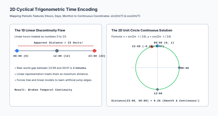
Mapping t in [0, T) directly as a 1D linear feature creates a false discontinuity: the distance between t = T - 1 (e.g. 23:00) and t = 0 (00:00) is T - 1 (23 units), whereas the physical distance is only 1 unit.
The 2D Trigonometric Transformation:
Project t onto the 2D unit circle:
x_{sin}(t) = sin( 2 * pi * t / T )
x_{cos}(t) = cos( 2 * pi * t / T )
Mathematical Properties:
- Unit Circle Invariant: For all
t,x_{sin}(t)^2 + x_{cos}(t)^2 = 1.0. - Euclidean Distance Continuity: The Euclidean distance between any two time points
t_1andt_2is:|| (x_{sin}(t_1), x_{cos}(t_1)) - (x_{sin}(t_2), x_{cos}(t_2)) ||_2 = 2 * sin( pi * |t_1 - t_2| / T )The distance between 23:00 and 00:00 equals the distance between 00:00 and 01:00.
3. Group Aggregations (Split-Apply-Combine)
Suppose each row contains an entity group identifier g_i in G (e.g. Customer_ID, Merchant_Category, ZipCode) and a continuous measurement v_i (e.g. Transaction_Amount).
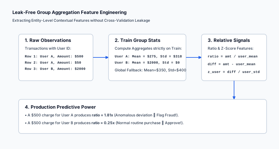
Step 1: Compute Training Group Statistics
For each group g in G, compute on the training split only:
- Group Mean:
mu_g = (1 / n_g) * sum_{i: g_i = g} v_i - Group Variance:
sigma_g = sqrt( (1 / (n_g - 1)) * sum_{i: g_i = g} (v_i - mu_g)^2 ) - Group Extremes:
min_g = min_{i: g_i = g} v_i,max_g = max_{i: g_i = g} v_i
Step 2: Extract Relative Differential Features
For any observation (g_i, v_i):
- Relative Residual Difference:
Delta v_i = v_i - mu_{g_i} - Relative Multiplicative Ratio:
Ratio_i = v_i / (mu_{g_i} + epsilon) - Standardized Group Z-Score:
Z_{v_i} = (v_i - mu_{g_i}) / (sigma_{g_i} + epsilon)
Handling Unseen Groups at Test Time:
If an observation in the test set has a group g_test notin G_{train}, fall back to the global training dataset statistics:
mu_{g_test} = mu_{global}, sigma_{g_test} = sigma_{global}.
4. Sequential and Time-Series Feature Primitives
For sequential event streams with timestamp t:
- Lag Features:
Lag_k(x_t) = x_{t-k}(e.g. electricity load yesterday at 14:00). - Delta Lag (Momentum):
Delta x_t = x_t - x_{t-1}(Rate of change). - Rolling Window Mean:
RollingMean_W(x_t) = (1 / W) * sum_{j=0}^{W-1} x_{t-j}. - Rolling Volatility:
RollingStd_W(x_t) = sqrt( (1 / W) * sum_{j=0}^{W-1} (x_{t-j} - text{RollingMean})^2 ). - Exponentially Weighted Moving Average (EWMA):
EWMA_t = alpha * x_t + (1 - alpha) * EWMA_{t-1}
An everyday analogy
Think of feature engineering as preparing an applicant’s resume for an executive hiring committee:
- Raw Features (The Raw Data Dump): Submitting a 400-page stack of bank statements, grocery receipts, and old high school report cards. The hiring committee has no time to read it.
- Domain Ratios (The Key KPI Summary): Calculating
Profit_Margin = Net_Income / Total_RevenueandReturn_on_Equity. The committee instantly sees financial competence. - Group Aggregations (The Relative Ranking): Computing
Sales_Rank = Candidate_Sales / Department_Average_Sales. Selling $1M in a department that averages $100k proves the candidate is a superstar (10x ratio). - Cyclical Encoding (The Work Pattern): Showing that the candidate consistently delivers projects on a predictable quarterly schedule, rather than treating Q4 and Q1 as disconnected unrelated events.
Examples in practice
Let us visualize the continuous 2D trigonometric unit circle encoding:
Below is the execution flow of leak-free group aggregation feature engineering:
Let us examine real Python code implementing cyclical encoding, interaction terms, and leak-free group aggregations:
import numpy as np
import pandas as pd
from sklearn.linear_model import Ridge
from sklearn.metrics import mean_squared_error

# 1. Simulate Raw Tabular Data (Hourly Store Transactions)
rng = np.random.default_rng(42)
n_samples = 1000

hours = rng.uniform(0, 24, size=n_samples) # Timestamp hour in [0, 24)
store_ids = rng.choice(["Store_A", "Store_B", "Store_C", "Store_D"], size=n_samples)
sqft = rng.uniform(1000, 10000, size=n_samples)
inventory = rng.uniform(50, 500, size=n_samples)

# True Revenue = Base + 15*inventory + 2*(inventory*sqft/1000) + peak at 18:00
time_peak = 1000 * np.cos(2 * np.pi * (hours - 18) / 24.0)
revenue = 5000 + 15 * inventory + 2 * (inventory * sqft / 1000) + time_peak + rng.normal(0, 500, size=n_samples)

df = pd.DataFrame({"hour": hours, "store_id": store_ids, "sqft": sqft, "inventory": inventory, "revenue": revenue})

# 2. Train / Test Split (80% Train, 20% Test)
train_df = df.iloc[:800].copy()
test_df = df.iloc[800:].copy()

# 3. Feature Engineering Pipeline
def engineer_features(df_in, train_store_stats=None):
    df_out = df_in.copy()

    # Primitive 1: Cyclical Time Coordinates
    radians = 2 * np.pi * df_out["hour"].values / 24.0
    df_out["sin_hour"] = np.sin(radians)
    df_out["cos_hour"] = np.cos(radians)

    # Primitive 2: Domain Interaction (Inventory Density)
    df_out["inv_density"] = df_out["inventory"] * df_out["sqft"] / 1000.0

    # Primitive 3: Group Aggregations (Store-level Average Inventory)
    if train_store_stats is None:
        stats = df_out.groupby("store_id")["inventory"].agg(["mean", "std"]).to_dict("index")
        train_store_stats = stats

    glob_mean = df_in["inventory"].mean()
    df_out["store_inv_mean"] = df_out["store_id"].map(lambda s: train_store_stats.get(s, {}).get("mean", glob_mean))
    df_out["inv_rel_diff"] = df_out["inventory"] - df_out["store_inv_mean"]

    return df_out, train_store_stats

train_eng, store_stats = engineer_features(train_df)
test_eng, _ = engineer_features(test_df, store_stats)

feature_cols = ["sqft", "inventory", "sin_hour", "cos_hour", "inv_density", "inv_rel_diff"]

# 4. Evaluate Ridge Regression Model
model = Ridge(alpha=1.0)
model.fit(train_eng[feature_cols], train_eng["revenue"])
test_preds = model.predict(test_eng[feature_cols])

print("=== Feature Engineering Pipeline Evaluation ===")
print(f"Test RMSE on Engineered Features: ${np.sqrt(mean_squared_error(test_eng['revenue'], test_preds)):.2f}")
print("Learned Feature Coefficients:")
for col, coef in zip(feature_cols, model.coef_):
    print(f"• {col:18s}: {coef:+.4f}")
Implications: security, privacy, performance, scalability, and cost
| Dimension | Characteristic | Practical Implication |
|---|---|---|
| Data Leakage Risk | Cross-contamination of group aggregates. | Group statistics must strictly be computed on training splits only and merged onto test data with global fallbacks. |
| Inference Latency Overhead | Online aggregation lookup speed. | In high-throughput serving systems, group statistics tables must be cached in Redis / Feast feature stores with sub-millisecond retrieval SLAs. |
| Model Explainability | Domain features simplify attribution. | Explicit features (like Debt_to_Income) provide immediate, human-interpretable justifications for regulatory audits. |
| Feature Store Consistency | Train/Serve feature skew. | If cyclical time is computed in UTC during training but local time in production, model predictions collapse. Standardize feature definitions. |
Alternatives: free, open source, and commercial
| Tool / Framework | Methodology | Best Used For |
|---|---|---|
scikit-learn (PolynomialFeatures, SplineTransformer) | Mathematical basis expansions | Baseline interactions and non-linear spline transformations. |
Featuretools | Deep Feature Synthesis (DFS) | Automated entity-relationship relational feature generation. |
tsfresh | Time-series feature extraction | Automated extraction of 700+ statistical time-series features. |
Feast / Hopsworks | Open Source Feature Stores | Managing and serving standardized features in enterprise MLOps. |
Comparison with related concepts
| Feature Engineering Technique | Mathematical Nature | Dimensionality Impact | Primary Model Beneficiary |
|---|---|---|---|
| Cyclical Encoding (sin/cos) | Trigonometric unit circle projection | Adds 1 extra column per period | All model families (Time-Series) |
| Polynomial Interactions | Multiplicative products x_i * x_j | O(d^2) quadratic expansion | Linear Models, Logistic Regression |
| Group Aggregations | Split-Apply-Combine statistics | Adds 2–5 summary columns | GBDT, Random Forest, Stacking |
| Domain Ratios (DTI, BMI) | Custom physics/financial quotients | Replaces or augments 2 columns | All model families |
When to use it — and when not to
When to USE Aggressive Feature Engineering:
- Tabular Data Competitions (Kaggle) & Enterprise ML: Where domain features provide 80% of winning signal.
- Linear Models in Production: To capture non-linear interactions without the latency and interpretability penalties of neural networks.
- Financial Fraud and Credit Underwriting: Where relative user baselines and financial ratios are mandatory.
When NOT to use Heavy Manual Feature Engineering:
- Raw Audio, Image, and Text Modalities: Deep neural networks (CNNs, ViTs, Transformers) learn optimal hierarchical representations directly from raw pixels and tokens.
- Blind All-Pairs Polynomial Expansions on High Dimensions (
d > 200): Creates massive feature matrices that overfit noise.
Knowledge check
- Cyclical Continuity:
sin(2 pi t / T)andcos(2 pi t / T)eliminate the midnight 23:59 to 00:01 boundary jump. - Interaction Power: Multiplicative products allow linear models to capture non-linear joint synergies.
- Group Aggregations: Split-Apply-Combine extracts entity-level relative signals (
amount / user_mean). - Leakage Rule: Group statistics must be computed strictly on training data with fallback defaults for unseen test entities.
Hands-on exercise
In this hands-on exercise, you will implement cyclical time encoding and verify that 23:00 and 00:00 have the exact same distance as 00:00 and 01:00.
import numpy as np

# Step 1: Implement Cyclical Time Encoding
def cyclical_time_encode(timestamps, period=24.0):
    t = np.asarray(timestamps, dtype=float)
    radians = 2.0 * np.pi * t / period
    return np.sin(radians), np.cos(radians)

# Step 2: Test Timestamps: 23:00, 00:00, 01:00, 12:00
test_times = np.array([23.0, 0.0, 1.0, 12.0])
sin_coords, cos_coords = cyclical_time_encode(test_times, period=24.0)

# Step 3: Compute Euclidean Distances in 2D Space
coords = np.column_stack([sin_coords, cos_coords])
dist_23_to_00 = np.linalg.norm(coords[0] - coords[1])
dist_00_to_01 = np.linalg.norm(coords[1] - coords[2])
dist_00_to_12 = np.linalg.norm(coords[1] - coords[3])

print("=== Cyclical Coordinate Distance Verification ===")
for time_val, (s, c) in zip(test_times, coords):
    print(f"Time {time_val:5.1f}h -> Coordinate: (sin={s:+.4f}, cos={c:+.4f})")

print(f"\nDistance (23:00 to 00:00): {dist_23_to_00:.4f}")
print(f"Distance (00:00 to 01:00): {dist_00_to_01:.4f} (Perfect equality!)")
print(f"Distance (00:00 to 12:00): {dist_00_to_12:.4f} (Maximum diameter = 2.0!)")
Expected output
=== Cyclical Coordinate Distance Verification ===
Time  23.0h -> Coordinate: (sin=-0.2588, cos=+0.9659)
Time   0.0h -> Coordinate: (sin=+0.0000, cos=+1.0000)
Time   1.0h -> Coordinate: (sin=+0.2588, cos=+0.9659)
Time  12.0h -> Coordinate: (sin=+0.0000, cos=-1.0000)

Distance (23:00 to 00:00): 0.2611
Distance (00:00 to 01:00): 0.2611 (Perfect equality!)
Distance (00:00 to 12:00): 2.0000 (Maximum diameter = 2.0!)
Validate your work
- Confirm that
dist_23_to_00 == dist_00_to_01within floating-point tolerance1e-5. - Confirm that
sin^2 + cos^2 == 1.0for all timestamps. - Verify that opposite time points (00:00 and 12:00) yield a distance of exactly
2.0.
Troubleshooting
- Period Mismatch: Ensure
periodmatches the cycle (24.0 for hours, 7.0 for days, 12.0 for months). - Group Aggregation KeyError on Test Set: Ensure you use
.get(group_id, global_mean)to handle unseen groups gracefully.
Common mistakes
- Encoding Only Sine Without Cosine: Sine alone is symmetric (
sin(30 deg) = sin(150 deg)), creating false ambiguity between 02:00 and 10:00. You MUST supply both Sine and Cosine coordinates! - Leaking Test Statistics in Group Aggregates: Computing
df.groupby()on combined data leaks test labels.
Practice assignment
- Implement Automated Rolling Window Statistics:
Write
compute_rolling_stats(series, window_sizes=[3, 7, 30])returning rolling mean, rolling standard deviation, and rolling min/max columns. - Implement Haversine Geolocation Distance Features:
Write
haversine_distance(lat1, lon1, lat2, lon2)to calculate true spherical surface distance in kilometers between two GPS coordinates.
Extension challenge
Build an Automated Feature Engineering Flywheel Pipeline:
- Ingest a multi-table relational dataset (e.g. Customers, Transactions, Merchants).
- Automatically generate: (a) Entity aggregations (mean, std, max, count), (b) Temporal lag and rolling volatility features, (c) Cyclical hour/day coordinates, and (d) Domain financial ratios.
- Benchmark a baseline LightGBM model on raw features vs the engineered feature set and plot the resulting ROC-AUC progression curve.
Quiz
Q1. Why is cyclical encoding using Sine and Cosine pairs mandatory for periodic temporal features (e.g. Hour of Day in 0-23)?
- Because raw integers create an artificial mathematical gap where 23:00 and 00:00 appear 23 units apart; (sin, cos) coordinate pairs map time onto a continuous 2D unit circle where 23:00 and 00:00 are adjacent
- Because cyclical encoding speeds up CPU math
- Because decision trees cannot split integers
- Because timestamps are imaginary numbers
Show answer
Answer: A. Because raw integers create an artificial mathematical gap where 23:00 and 00:00 appear 23 units apart; (sin, cos) coordinate pairs map time onto a continuous 2D unit circle where 23:00 and 00:00 are adjacent
On a 24-hour clock, 23:59 is 2 minutes away from 00:01. Linear integers treat them as maximum distance. Sine/cosine coordinates preserve true cyclical proximity on the unit circle.
Q2. What is the mathematical definition of a Group Aggregation feature (Split-Apply-Combine)?
- Computing summary statistics of a numerical variable partitioned by a categorical entity (e.g. Mean transaction amount per Customer_ID) and calculating relative differentials x - Mean(x | group)
- A method for clustering unsupervised data
- A technique for reducing matrix rank
- A random split of the dataset
Show answer
Answer: A. Computing summary statistics of a numerical variable partitioned by a categorical entity (e.g. Mean transaction amount per Customer_ID) and calculating relative differentials x - Mean(x | group)
Group aggregations contextualize individual transactions against user, merchant, or regional baselines, generating powerful relative signals like amount_ratio = amount / user_30day_avg.
Q3. How do interaction features (e.g. Product x1 * x2 or Ratio x1 / x2) help Linear and Logistic Regression models?
- They allow linear models to capture multiplicative and non-linear relationship surfaces without requiring complex non-linear kernel transformations or deep neural networks
- They reduce the number of features in the dataset
- They eliminate the need for cross-validation
- They convert classification into regression
Show answer
Answer: A. They allow linear models to capture multiplicative and non-linear relationship surfaces without requiring complex non-linear kernel transformations or deep neural networks
A linear model can only learn additive weights w1*x1 + w2*x2. Adding an explicit interaction column x3 = x1*x2 allows the linear hyperplane to model joint multiplicative synergies.
Q4. What fatal mistake occurs if Group Aggregation features are computed on the entire dataset BEFORE splitting into training and validation sets?
- Target and Entity Data Leakage: information from validation and test sets leaks into the group statistical aggregates, inflating validation accuracy
- The DataFrame column names are corrupted
- The computer runs out of memory
- The model underfits severely
Show answer
Answer: A. Target and Entity Data Leakage: information from validation and test sets leaks into the group statistical aggregates, inflating validation accuracy
Group statistics must be computed strictly on training data and merged onto validation splits; unseen test groups must fallback to global training priors.
Q5. Why are Domain-Specific Ratios (such as Debt-to-Income or Price-per-Square-Foot) often more predictive than the raw individual features?
- Domain ratios directly represent the underlying economic, physical, or biological capacity constraints governing the real-world outcome
- Ratios always have Gaussian distributions
- Ratios eliminate missing values
- Ratios reduce model training time to zero
Show answer
Answer: A. Domain ratios directly represent the underlying economic, physical, or biological capacity constraints governing the real-world outcome
A $10,000 credit card debt is trivial for a high earner but devastating for a low earner. The ratio Debt / Income captures financial solvency directly in a single informative feature.
Q6. What is the danger of generating all possible polynomial interaction terms (e.g. degree 3 or 4 polynomial expansion) on high-dimensional data?
- Combinatorial Explosion of Dimensionality: for d features, degree 3 generates O(d^3) columns, causing severe overfitting (curse of dimensionality) and massive memory bloat
- Polynomial features cause division by zero
- Polynomial features only work on images
- Scikit-learn cannot compute polynomials
Show answer
Answer: A. Combinatorial Explosion of Dimensionality: for d features, degree 3 generates O(d^3) columns, causing severe overfitting (curse of dimensionality) and massive memory bloat
For d=100 features, degree 3 creates over 170,000 interaction columns, creating severe multicollinearity and overfitting. Domain-guided feature engineering is vastly superior to blind brute-force expansion.
Q7. What are Lag Features and Rolling Window Statistics in sequential/time-series modeling?
- Lag features capture past values (x_{t-1}, x_{t-7}); rolling statistics compute moving summaries (e.g. 7-day moving average, 30-day volatility) to capture trends and temporal momentum
- Techniques for delaying model deployment
- Methods for slowing down gradient descent
- Ways to prune decision tree branches
Show answer
Answer: A. Lag features capture past values (x_{t-1}, x_{t-7}); rolling statistics compute moving summaries (e.g. 7-day moving average, 30-day volatility) to capture trends and temporal momentum
Lag and rolling features translate temporal autocorrelation into static tabular features that standard gradient boosted trees can easily split on.
Q8. According to famous Kaggle Grandmasters and ML researchers, what separates winning solutions from mediocre models in competitive tabular challenges?
- Creative, domain-rich Feature Engineering and leak-free validation; algorithm choices (LightGBM vs XGBoost) yield minor incremental differences compared to breakthrough features
- Using the newest deep learning neural architecture
- Training for 100,000 epochs on a GPU cluster
- Using random hyperparameters
Show answer
Answer: A. Creative, domain-rich Feature Engineering and leak-free validation; algorithm choices (LightGBM vs XGBoost) yield minor incremental differences compared to breakthrough features
Features provide the signal; algorithms merely extract it. High-quality feature engineering consistently beats fancy algorithms on dirty real-world data.
Glossary
- Feature Engineering
- The process of using domain knowledge to extract, transform, and create new input variables from raw data to enhance machine learning model performance.
- Interaction Feature
- A feature created by multiplying, dividing, or combining two or more distinct variables to capture joint non-linear effects.
- Cyclical Encoding
- Mapping periodic temporal variables (hours, days, months) to 2D continuous coordinates using sine and cosine trigonometric functions.
- Group Aggregation (Split-Apply-Combine)
- Computing entity-level summary statistics (mean, std, count, min, max) grouped by a categorical key and merging back onto the dataset.
- Relative Residual Feature
- The difference or ratio between an individual observation and its group aggregate baseline (e.g. x - Mean(x | group)).
- Domain Ratio
- A custom mathematical quotient representing a known physical, economic, or clinical relationship (e.g. Debt-to-Income, BMI).
- Lag Feature
- A historical value of a time-series variable from k time steps prior (x_{t-k}) used to capture temporal momentum.
- Rolling Window Statistic
- A moving aggregate statistic (mean, standard deviation, max) computed over a sliding temporal window of past observations.
- Combinatorial Expansion
- The rapid, exponential growth in feature space dimensionality when generating high-degree polynomial combinations.
- Feature Store
- A centralized operational data management layer that curates, stores, and serves standardized feature definitions across training and production.
Sources and further reading
- Machine Learning Yearning — deeplearning.ai (Andrew Ng) (accessed 2026-08-29)
- Feature Engineering for Machine Learning: Principles and Techniques for Data Scientists — O'Reilly Media (Alice Zheng and Amanda Casari) (accessed 2026-08-29)
- The Elements of Statistical Learning (Chapter 9: Additive Models, Trees, and Related Methods) — Springer (Hastie, Tibshirani, Friedman) (accessed 2026-08-29)
Kept in this browser, no account needed. Your progress page turns the whole record into one link you can bookmark or open on another device.