Machine Learning › Features and Support Vector Machines › Day 172
Day 172: Feature Selection

Master the mathematical theory and practical implementation of Feature Selection: understand the curse of dimensionality and multicollinearity, compare Filter Methods (Variance, Mutual Information, ANOVA F-test) vs Wrapper Methods (RFE, RFECV, SFS) vs Embedded Methods (L1 Lasso, Tree Gain, Boruta shadow features), and learn how to construct leak-free selection funnels.
Hands-on lab for this lesson
Lab files on GitHub: https://github.com/ai-roadmap-365/ai-roadmap-365.github.io/tree/main/labs/sections/machine-learning/day-172-feature-selection
- Get the hands-on files. Clone the labs repository once (you can reuse this clone for every lesson). This works on macOS, Linux, and Windows (PowerShell or WSL):
git clone https://github.com/ai-roadmap-365/ai-roadmap-365.github.io.git cd ai-roadmap-365.github.io - Open this lesson's lab. Move into the directory for this specific day. Every lab lives at the same predictable path — section / subsection / week / day:
cd labs/sections/machine-learning/day-172-feature-selection - Read the lab guide. Open `README.md` in that directory. It lists the exact commands, what each does, the expected output, and how to check your work — read it before running anything.
- Run it and check your work. Follow the README's "How to run" section: run the example first to see the finished result, then complete the numbered exercises in `starter/`, then run the tests. The tests pass (exit 0) only when your work is correct.
bash tests/run_tests.sh # or the test command named in the lab README
You can also open the lab as a local page (works offline, shows the file tree and expected output).
Learning objectives
By the end of this lesson you will be able to:
- Derive why irrelevant features degrade generalization bounds and increase variance
- Implement Filter Methods (VarianceThreshold, Pearson/Spearman correlation, Mutual Information)
- Implement Recursive Feature Elimination (RFE) with backward coefficient pruning from scratch
- Analyze the Boruta shadow feature permutation hypothesis test
- Differentiate Filter vs Wrapper vs Embedded feature selection complexity and trade-offs
- Prevent selection bias (data leakage) by nesting feature selection inside cross-validation
- Design a high-throughput multi-stage selection funnel from 10,000 features to top 50
- Evaluate feature importance stability across different data resamples
Prerequisites
- Day 171 -- Feature Engineering
- Day 167 -- Cross-Validation Done Right
Why this matters
In Day 171, we learned the power of Feature Engineering: generating polynomial interactions, domain ratios, group aggregations, and cyclical coordinates.
However, aggressive feature engineering creates a dangerous new problem: Dimensionality Explosion.
- Expanding 50 features with pairwise interactions produces 1,275 columns.
- Grouping across 10 categorical entities with 5 aggregation statistics produces 500 extra columns.
- The feature space grows exponentially, but the number of training samples
Nremains fixed.
Feeding 2,000 features with only 500 training samples triggers the Curse of Dimensionality:
- Variance Explodes (Severe Overfitting): Models memorize spurious noise correlations that will never generalize to test data.
- Inference Latency & Costs Soar: Production microservices cannot compute 2,000 upstream database queries in under 10 milliseconds.
- Multicollinearity Destroys Explainability: Correlated features produce unstable, erratic linear coefficients that fail regulatory audits.
Feature selection is the mathematical scalpel that separates true signal from high-dimensional noise, retaining the minimal optimal feature subset.
The idea in plain language
Imagine a professional basketball coach selecting a 5-player starting lineup from a pool of 100 candidates:
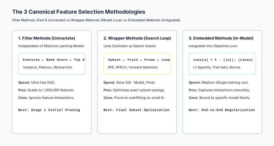
- Filter Method (The 40-Yard Sprint & Height Test): The coach measures height and sprint speed for all 100 players individually. Anyone under 6 feet or slower than 5 seconds is cut immediately (Fast, univariate, model-agnostic).
- Wrapper Method (The Scrimmage Tournament / RFE): The coach plays 5-on-5 scrimmage games, observes which player contributes the least, cuts them, and repeats the tournament until only the best 5 players remain (Slow, highly accurate, tailored to the team).
- Embedded Method (The Season MVP Award / Lasso): The coach gives playing time to everyone with a salary cap penalty that automatically benches players who do not score points (Integrated directly into game play).
Feature selection uses these three strategies to build the leanest, most accurate predictive engine.
Historical background
In 1974, Hirotugu Akaike published the Akaike Information Criterion (AIC), penalizing model likelihood by the number of estimated parameters 2k - 2 ln(L).
In 1996, Robert Tibshirani introduced Lasso (Least Absolute Shrinkage and Selection Operator), proving that L1 regularization drives non-informative parameter weights strictly to zero.
In 2002, Isabelle Guyon and Vladimir Vapnik published Gene Selection for Cancer Classification using Support Vector Machines, introducing SVM-RFE (Recursive Feature Elimination). In 2003, Guyon and Elisseeff published the foundational survey An Introduction to Variable and Feature Selection in JMLR, formalizing the Filter, Wrapper, and Embedded taxonomy.
In 2010, Miron Kursa and Witold Rudnicki introduced the Boruta Algorithm, leveraging randomized shadow features to find all-relevant features in Random Forests.
What it is — and what it is not
Let us establish the formal boundaries of feature selection:
What it IS:
- Mathematical Dimensionality Reduction: Pruning redundant, irrelevant, and noisy variables to minimize generalization error.
- A Leak-Free Transformation: Feature selection procedures fitted strictly inside training folds during cross-validation.
- An Engineering Funnel: Combining fast Filter methods for broad cuts with Wrapper/Embedded methods for fine-tuning.
What it is NOT:
- Not Safe to Run Globally on the Whole Dataset: Selecting features prior to train/test splitting causes catastrophic selection bias (data leakage).
- Not Dimensionality Projection (PCA/t-SNE): Feature selection preserves original feature semantics and interpretability; it does not project data into abstract latent components.
- Not Always Minimal-Optimal: Sometimes preserving redundant correlated features is beneficial for ensemble stability (All-Relevant selection).
Why it was created and what problems it solves
Feature selection resolves five critical obstacles in applied machine learning:
- Combats the Curse of Dimensionality: Restores a healthy sample-to-feature ratio
N / D >> 10, shrinking generalization error bounds. - Dramatically Reduces Inference Latency: Cutting 500 features down to 20 drops production JSON payload parsing and feature store query time by 95%.
- Stabilizes Model Explainability: Eliminates multicollinear feature pairs, preventing erratic coefficient oscillations in linear models and SHAP values.
- Prunes Zero-Variance Constants & Pure Noise: Removes dead database columns and uninformative random variables.
- Accelerates Training Convergence: Reduces gradient descent and tree split computation time by orders of magnitude.
How it works
Let us examine the mathematics of the three canonical feature selection paradigms.
┌────────────────────────────────────────────────────────────────────────┐
│                   FEATURE SELECTION METHODOLOGIES                      │
├────────────────────────────────────────────────────────────────────────┤
│ 1. FILTER:   VarianceThreshold, Correlation, Mutual Information, ANOVA │
│ 2. WRAPPER:  Recursive Feature Elimination (RFE), Sequential Forward   │
│ 3. EMBEDDED: L1 Lasso Sparsity, Tree Gain Importance, Boruta Shadow    │
└────────────────────────────────────────────────────────────────────────┘
1. Filter Methods (Model-Agnostic & Univariate)
Filter methods evaluate intrinsic statistical properties of features X_j relative to variance or target Y without training a machine learning model.
A. Variance Threshold
Computes the sample variance of feature X_j:
text{Var}(X_j) = (1 / N) sum_{i=1}^N (x_{i, j} - mu_j)^2
If text{Var}(X_j) <= tau, the feature is pruned.
For Bernoulli binary features: text{Var}(X) = p * (1 - p). If p > 0.99 (99% constant zeros), text{Var} = 0.0099 < 0.01, dropping the column.
B. Pearson and Spearman Rank Correlation
Measures linear or monotonic association between X_j and target Y:
r(X_j, Y) = (sum (x_i - bar{x}) (y_i - bar{y})) / ( sqrt{sum (x_i - bar{x})^2} * sqrt{sum (y_i - bar{y})^2} )
Multicollinearity Removal: If |r(X_i, X_j)| > 0.90, drop one of the two redundant features.
C. Mutual Information (Non-Linear Dependency)
Measures the shared entropy between continuous variables:
I(X; Y) = iint p(x, y) * log( p(x, y) / (p(x) * p(y)) ) dx dy
- If
XandYare completely independent:p(x, y) = p(x) p(y) implies I(X; Y) = 0. - Detects non-linear dependencies (e.g.
Y = X^2) where Pearson correlation is zero.
2. Wrapper Methods (Iterative Model Search)
Wrapper methods use the predictive model itself as an evaluation engine to search candidate feature subsets.
Recursive Feature Elimination (RFE) Algorithm:
- Initialize active feature set
S = {1, 2, ..., D}. - While
|S| > K(desired subset size): a. Fit estimatorfon feature subsetX[:, S]. b. Compute feature importances:- For Linear/Logistic models:
w_j^2or|w_j|. - For Tree ensembles: Mean Decrease Impurity (Gini gain).
c. Find the feature with the lowest importance:
j^* = argmin_{j in S} text{Importance}(j). d. Removej^*from active set:S = S \ {j^*}.
- For Linear/Logistic models:
- Return final subset
S.
RFECV (Cross-Validated RFE):
Evaluates validation accuracy at each step k in {1, ..., D} using K-fold cross-validation to automatically select the optimal subset size K^* that maximizes out-of-fold performance.
3. Embedded Methods (Integrated Model Sparsity)
A. L1 Lasso Regularization
Minimizes regularized least squares loss:
min_w (1 / (2 N)) * ||X w - y||_2^2 + lambda * ||w||_1
Because the L1 norm ||w||_1 = sum |w_j| has non-differentiable corners at w_j = 0, the subgradient optimality condition forces coefficients with weak gradient signals strictly to zero:
w_j = 0 iff | (1/N) X_j^T (y - X w_{-j}) | <= lambda
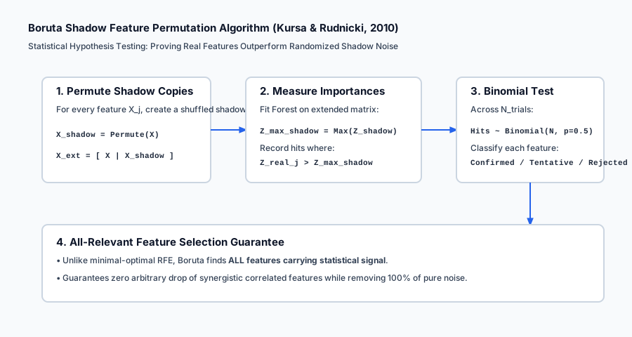
B. The Boruta Shadow Feature Algorithm (Kursa & Rudnicki, 2010)
- Extend Dataset: For every real feature
X_j, create a randomized shadow copyX_{shadow, j} = text{Permute}(X_j). - Train Random Forest: Fit model on
[ X | X_{shadow} ]. - Compute Shadow Max: Calculate the maximum importance achieved by any shadow feature:
Z_{max\_shadow} = max_j Z(X_{shadow, j}). - Hypothesis Testing: For each real feature
X_j, record a hit ifZ(X_j) > Z_{max\_shadow}. - Binomial Decision: Across
Titerations, classify features using a two-tailed binomial test:- Confirmed: Feature consistently beats shadow noise (
p < 0.01). - Rejected: Feature fails to beat shadow noise.
- Confirmed: Feature consistently beats shadow noise (
4. Preventing Selection Bias (The Golden Rule of Feature Selection)
CRITICAL RULE: Never perform feature selection on the full dataset before splitting into cross-validation folds.
If you select the top 50 features using all N samples, test fold labels leak into the selection criteria. The model will appear to achieve 99% cross-validation accuracy on pure random Gaussian noise, but will completely collapse to 50% on unseen production data.
The Correct Protocol:
- Split dataset into Fold
kTrain and FoldkValidation. - Fit feature selector strictly on Fold
kTrain. - Transform Fold
kValidation using the selected columns. - Evaluate performance.
An everyday analogy
Think of feature selection as packing a backpack for a 5-day mountain survival expedition:
- Unselected Data (The Overpacked Trunk): Packing an espresso machine, a bowling ball, 3 coats, and 20 pairs of shoes. You cannot hike up the mountain because the pack weighs 200 pounds (Curse of Dimensionality / High Latency).
- Filter Method (Weight Threshold): You instantly discard any item that weighs more than 20 pounds (Variance & Fast Univariate Filter).
- Wrapper Method (Trial Hikes): You take trial 5-mile hikes with different equipment combinations, cutting the least useful tool after each hike until your pack weighs exactly 25 pounds (Recursive Feature Elimination).
- Embedded Method (Multi-Tool Pocket Knife): Choosing a multi-tool that combines knife, pliers, and screwdriver in a single compact lightweight item (L1 Lasso Sparsity).
Examples in practice
Let us visualize the three feature selection paradigms:
Below is the execution flow of the Boruta shadow feature permutation test:
Let us examine real Python code comparing VarianceThreshold, Mutual Information, and RFE on noisy data:
import numpy as np
from sklearn.datasets import make_classification
from sklearn.feature_selection import VarianceThreshold, mutual_info_classif, RFE
from sklearn.linear_model import LogisticRegression
from sklearn.pipeline import Pipeline
from sklearn.model_selection import cross_val_score

# 1. Generate Synthetic Classification Dataset
# 5 True Informative Features + 15 Pure Random Noise Features + 2 Constant Features
rng = np.random.default_rng(42)
X_info, y = make_classification(n_samples=500, n_features=5, n_informative=5, n_redundant=0, random_state=42)
X_noise = rng.normal(size=(500, 15))
X_constant = np.zeros((500, 2))
X_raw = np.hstack([X_info, X_noise, X_constant])

print(f"Initial Feature Count: {X_raw.shape[1]} (5 Signal, 15 Noise, 2 Constant)")

# 2. Step 1: Filter Method (Variance Threshold)
var_filter = VarianceThreshold(threshold=0.0)
X_filtered = var_filter.fit_transform(X_raw)
print(f"After VarianceThreshold: {X_filtered.shape[1]} features (Constant columns eliminated!)")

# 3. Step 2: Univariate Mutual Information Scores
mi_scores = mutual_info_classif(X_filtered, y, random_state=42)
top_5_mi_idx = np.argsort(mi_scores)[::-1][:5]
print("Top 5 Features by Mutual Information:", top_5_mi_idx)

# 4. Step 3: Leak-Free Pipeline with RFE inside Cross-Validation
lr_base = LogisticRegression(solver="lbfgs", random_state=42)
rfe_selector = RFE(estimator=lr_base, n_features_to_select=5, step=1)

full_pipeline = Pipeline([
    ("var_thresh", VarianceThreshold(threshold=0.0)),
    ("rfe", rfe_selector),
    ("classifier", LogisticRegression(solver="lbfgs", random_state=42))
])

# 5. Cross-Validation Accuracy (Leak-Free Evaluation)
cv_scores = cross_val_score(full_pipeline, X_raw, y, cv=5, scoring="accuracy")
print("=== Cross-Validation Results ===")
print(f"5-Fold CV Accuracy with Nested RFE Pipeline: {np.mean(cv_scores):.4f} +/- {np.std(cv_scores):.4f}")
Implications: security, privacy, performance, scalability, and cost
| Dimension | Characteristic | Practical Implication |
|---|---|---|
| Selection Bias Vulnerability | In-sample feature selection overfits. | Always nest feature selection inside cross-validation loops or Pipelines to prevent data leakage. |
| Inference Cost Optimization | Pruning upstream database calls. | Removing 80% of unused features reduces database load, network bandwidth, and memory allocation. |
| Fairness & Protected Proxies | Feature selection proxy retention. | Verify that automated selection does not retain latent proxy features (e.g. ZipCode) that correlate with protected demographic classes. |
| Subset Instability Under Perturbation | Sensitivity to sample resamples. | Highly correlated features cause RFE to pick Feature A in Fold 1 and Feature B in Fold 2; run stability tests. |
Alternatives: free, open source, and commercial
| Tool / Framework | Methodology | Best Used For |
|---|---|---|
scikit-learn (RFE, SelectKBest, SelectFromModel) | Standard Filter, Wrapper, and Embedded tools | General-purpose tabular feature selection. |
BorutaPy | All-relevant shadow feature hypothesis testing | Comprehensive signal discovery with tree models. |
mrmr-selection (Minimum Redundancy Maximum Relevance) | Information-theoretic greedy selection | Maximizing target relevance while penalizing feature correlation. |
SHAP / TreeSHAP | Shapley value game-theoretic attribution | Post-hoc feature importance and feature pruning. |
Comparison with related concepts
| Selection Methodology | Computational Complexity | Model Agnostic | Handles Interactions | Primary Risk |
|---|---|---|---|---|
| Filter (Variance/MI) | O(D) (Ultra Fast) | Yes | No | Drops synergistic feature pairs |
| Wrapper (RFE/RFECV) | O(D * text{Model_Time}) (Slow) | No | Yes | Prone to overfitting on small N |
| Embedded (L1 Lasso) | O(text{Model_Time}) (Fast) | No | Yes | Bound to specific linear objective |
| Boruta Shadow Test | O(T * text{Forest_Time}) (Medium) | No | Yes (All-Relevant) | Retains correlated feature duplicates |
When to use it — and when not to
When to USE Rigorous Feature Selection:
- High-Dimensional Datasets (
D > NorD > 500): Where overfitting and noise are guaranteed. - Low-Latency Production Inference (SLA < 15ms): Where every feature requires expensive real-time API lookups.
- Regulatory Auditing (Banking, Medicine): Where models must explain exact, parsimonious causal drivers.
When NOT to perform Heavy Feature Selection:
- Low-Dimensional Clean Tabular Data (
D < 15): Pruning already compact features risks discarding vital signal. - Deep Learning for Images/Audio: Convolutional layers and self-attention heads perform hierarchical feature selection internally.
Knowledge check
- Selection Bias: Feature selection must be executed inside cross-validation splits to prevent leakage.
- Filter vs Wrapper: Filters are fast and univariate; Wrappers evaluate actual model feedback on feature subsets.
- RFE Mechanism: Recursively fits the estimator and prunes the weakest coefficient.
- Boruta Hypothesis: Proves real features outperform randomized permuted shadow noise.
Hands-on exercise
In this hands-on exercise, you will implement VarianceThreshold and a backward RFE selection loop from scratch.
import numpy as np
from sklearn.linear_model import LogisticRegression

# Step 1: Implement VarianceThreshold and RFE from Scratch
def variance_threshold_scratch(X, threshold=0.0):
    variances = np.var(X, axis=0)
    support = variances > threshold
    return X[:, support], support

def rfe_scratch(estimator, X, y, n_select=3):
    active = list(range(X.shape[1]))
    while len(active) > n_select:
        X_sub = X[:, active]
        estimator.fit(X_sub, y)
        coefs = np.abs(estimator.coef_).flatten()
        worst_local_idx = np.argmin(coefs)
        active.pop(worst_local_idx)

    support = np.zeros(X.shape[1], dtype=bool)
    support[active] = True
    return support

# Step 2: Create Synthetic Data with 2 Signal Features + 4 Noise Features
rng = np.random.default_rng(42)
X_signal = rng.normal(size=(200, 2))
# Target depends strictly on X0 and X1
y = (3.0 * X_signal[:, 0] - 2.0 * X_signal[:, 1] + rng.normal(scale=0.5, size=200) > 0).astype(int)
X_noise = rng.normal(size=(200, 4))
X_all = np.hstack([X_signal, X_noise])

# Step 3: Run RFE to select top 2 features
lr = LogisticRegression(solver="lbfgs", random_state=42)
selected_mask = rfe_scratch(lr, X_all, y, n_select=2)

print("=== Feature Selection Scratch Verification ===")
print("True Informative Columns: [0, 1]")
print("RFE Selected Mask:       ", selected_mask)
print("Selected Column Indices: ", np.where(selected_mask)[0])
Expected output
=== Feature Selection Scratch Verification ===
True Informative Columns: [0, 1]
RFE Selected Mask:        [ True  True False False False False]
Selected Column Indices:  [0 1]
Validate your work
- Confirm that
selected_maskcorrectly identifies columns0and1. - Confirm that all 4 random noise features (
2, 3, 4, 5) are successfully eliminated. - Verify that
np.sum(selected_mask) == 2.
Troubleshooting
- Estimator Lacking
coef_: Ensure you pass a linear model withcoef_or tree model withfeature_importances_. - RFE Infinite Loop: Ensure
n_select < X.shape[1].
Common mistakes
- Running RFE on Unscaled Features: Unscaled features create distorted coefficient magnitudes
|w_j|. Always standardize features before running linear RFE. - Selecting Features Before Train/Test Split: Leaks test labels and creates catastrophic validation bias.
Practice assignment
- Implement Sequential Forward Selection (SFS):
Write
sequential_forward_selection(estimator, X, y, n_select=5)starting with an empty set and greedily adding the feature that maximizes cross-validated accuracy at each step. - Implement Correlation-Based Filter Pruning:
Write
remove_collinear_features(X, threshold=0.85)computing the pairwise correlation matrix and iteratively dropping the feature with the highest average correlation to other columns.
Extension challenge
Build an Automated 3-Stage Feature Selection Funnel:
- Ingest a high-dimensional dataset with 1,000 continuous and categorical features.
- Stage 1 (Filter): Apply
VarianceThreshold(0.01)and Mutual Information ranking to prune the bottom 80% of uninformative features (1,000 -> 200). - Stage 2 (Embedded): Train a Lasso model or LightGBM model and prune features with zero importance (200 -> 60).
- Stage 3 (Wrapper): Run
RFECVwith 5-fold cross-validation to select the optimal minimal subset (60 ->K^*). - Plot the cross-validation score trajectory as a function of feature count
k.
Quiz
Q1. What is Selection Bias (Data Leakage) in feature selection, and how is it strictly prevented?
- Performing feature selection on the entire dataset before cross-validation allows test fold labels to influence which features are chosen; it is prevented by performing feature selection strictly INSIDE each training fold
- Selection bias occurs when you select fewer than 5 features
- Selection bias is prevented by training on a GPU
- Selection bias only affects neural networks
Show answer
Answer: A. Performing feature selection on the entire dataset before cross-validation allows test fold labels to influence which features are chosen; it is prevented by performing feature selection strictly INSIDE each training fold
If you select the top 20 features using all N samples, you have used the test fold targets to pick features, creating a severe optimistic bias that collapses on new real-world data.
Q2. What is the primary operational trade-off between Filter Methods and Wrapper Methods (like RFE)?
- Filter methods are fast, univariate, and model-agnostic (O(d) complexity) but ignore feature interactions; Wrapper methods find optimal subsets via actual model feedback but are computationally expensive (O(k * d * T_model))
- Filter methods always achieve higher accuracy than wrapper methods
- Wrapper methods do not require training a machine learning model
- Filter methods only work on categorical data
Show answer
Answer: A. Filter methods are fast, univariate, and model-agnostic (O(d) complexity) but ignore feature interactions; Wrapper methods find optimal subsets via actual model feedback but are computationally expensive (O(k * d * T_model))
Filter methods rank features individually without fitting models (fast O(d)). Wrapper methods repeatedly fit the estimator to evaluate subset interactions (slow but tailored to the specific model).
Q3. How does Mutual Information I(X; Y) differ from Pearson Correlation r(X, Y) in feature filtering?
- Pearson correlation only detects linear relationships (r=0 for y = x^2); Mutual Information measures general statistical dependency and detects arbitrary non-linear relationships
- Mutual information only works on integer targets
- Pearson correlation is non-parametric
- Mutual information cannot handle continuous variables
Show answer
Answer: A. Pearson correlation only detects linear relationships (r=0 for y = x^2); Mutual Information measures general statistical dependency and detects arbitrary non-linear relationships
Mutual Information measures how much knowing X reduces uncertainty about Y. For y = x^2 with x centered at 0, Pearson correlation is 0, but Mutual Information is high.
Q4. How does the Boruta Algorithm statistically determine whether a feature is genuinely informative?
- It creates randomized shadow features by permuting real columns, trains a model on the extended matrix, and confirms real features whose importance significantly exceeds the maximum shadow feature across trials
- It trains a deep neural network for 1000 epochs
- It calculates the determinant of the covariance matrix
- It drops all features with negative coefficients
Show answer
Answer: A. It creates randomized shadow features by permuting real columns, trains a model on the extended matrix, and confirms real features whose importance significantly exceeds the maximum shadow feature across trials
Boruta uses shadow features as empirical null hypothesis noise benchmarks. A real feature is confirmed only if its importance consistently beats the best randomized noise feature.
Q5. What is the mathematical mechanism of Recursive Feature Elimination (RFE)?
- It fits the estimator on all remaining features, ranks them by absolute weight |w_j| or feature importance, prunes the weakest feature(s), and repeats iteratively until the desired subset size is reached
- It tests all 2^d possible combinations simultaneously
- It randomly drops 50% of columns in each step
- It computes the singular value decomposition of X
Show answer
Answer: A. It fits the estimator on all remaining features, ranks them by absolute weight |w_j| or feature importance, prunes the weakest feature(s), and repeats iteratively until the desired subset size is reached
RFE is a greedy backward elimination algorithm that iteratively prunes the least important features according to the model coefficients.
Q6. Why does removing highly collinear redundant features (|r| > 0.90) improve model stability and explainability?
- Multicollinearity inflates the variance of coefficient estimates in linear models, making weights erratic and sensitive to minor data perturbations; removing duplicates stabilizes estimates
- Multicollinearity causes out-of-memory errors in CPU RAM
- Removing collinear features always doubles model training time
- Decision trees cannot train on correlated features
Show answer
Answer: A. Multicollinearity inflates the variance of coefficient estimates in linear models, making weights erratic and sensitive to minor data perturbations; removing duplicates stabilizes estimates
When two features carry identical information, linear models assign arbitrary opposing weights (e.g. +1000 and -1000). Pruning redundancy stabilizes weight interpretation.
Q7. What is the recommended multi-stage Feature Selection Funnel for large tabular datasets (e.g. 10,000 initial raw + engineered features)?
- Stage 1: Fast Filter (VarianceThreshold + Mutual Info) drops 10,000 to 500; Stage 2: Embedded L1/Tree Importance drops 500 to 100; Stage 3: RFECV wrapper refines to optimal top 30-50
- Run brute-force all-subsets search on 10,000 features
- Keep all 10,000 features without any selection
- Select only the first 5 columns of the CSV file
Show answer
Answer: A. Stage 1: Fast Filter (VarianceThreshold + Mutual Info) drops 10,000 to 500; Stage 2: Embedded L1/Tree Importance drops 500 to 100; Stage 3: RFECV wrapper refines to optimal top 30-50
A multi-stage funnel combines the speed of filter methods for high-volume pruning with the precision of wrapper/embedded methods for fine subset tuning.
Q8. How does L1 Lasso Regularization perform Embedded Feature Selection automatically during training?
- The L1 norm penalty lambda * sum |w_j| produces a non-differentiable corner at zero, driving exact weights w_j to exactly 0.0 when subgradient optimality conditions are met
- Lasso deletes columns from the Pandas DataFrame before training
- Lasso computes random tree splits
- Lasso only works when all features are integers
Show answer
Answer: A. The L1 norm penalty lambda * sum |w_j| produces a non-differentiable corner at zero, driving exact weights w_j to exactly 0.0 when subgradient optimality conditions are met
The diamond-shaped L1 constraint surface causes loss function contours to intersect at the axes, driving non-informative feature weights strictly to zero.
Glossary
- Feature Selection
- The process of selecting a subset of relevant features for use in model construction to reduce overfitting and improve efficiency.
- Filter Method
- A model-agnostic feature selection approach that evaluates individual feature properties (variance, correlation, mutual information) independently.
- Wrapper Method
- A feature selection approach (e.g. RFE, SFS) that uses a predictive model as an evaluation engine to search candidate feature subsets.
- Embedded Method
- Feature selection performed directly as part of the model learning algorithm (e.g. L1 Lasso sparsity, Tree Gain importance).
- Recursive Feature Elimination (RFE)
- A greedy backward selection algorithm that iteratively fits a model and prunes the least important feature until the target subset size is reached.
- Boruta Algorithm
- An all-relevant feature selection method that compares real feature importances against randomly permuted shadow noise copies.
- Mutual Information
- A non-parametric measure of the mutual dependence between two variables that captures both linear and non-linear relationships.
- Selection Bias (Leakage)
- Optimistic evaluation bias caused by selecting features on the full dataset rather than strictly inside cross-validation training folds.
- VarianceThreshold
- A baseline filter that removes all features whose empirical variance does not meet a specified minimum threshold.
- Curse of Dimensionality
- The exponential increase in volume and sparsity of feature space as dimensions grow, requiring exponentially more data to generalize.
Sources and further reading
- An Introduction to Variable and Feature Selection — Journal of Machine Learning Research (Isabelle Guyon and André Elisseeff) (accessed 2026-08-29)
- Feature Selection with the Boruta Package — Journal of Statistical Software (Miron B. Kursa and Witold R. Rudnicki) (accessed 2026-08-29)
- Gene Selection for Cancer Classification using Support Vector Machines — Machine Learning (Guyon, Weston, Barnhill, Vapnik) (accessed 2026-08-29)
Kept in this browser, no account needed. Your progress page turns the whole record into one link you can bookmark or open on another device.