Deep Learning › Training Deep Networks › Day 206
Day 206: Optimizers: SGD to Adam
Master deep learning optimization algorithms: trace the mathematical evolution from vanilla SGD to Polyak Momentum, Nesterov acceleration, AdaGrad, RMSprop, Adam, and AdamW, implement custom optimizers from scratch, and choose the optimal optimizer and hyperparameters in PyTorch.
Hands-on lab for this lesson
Lab files on GitHub: https://github.com/ai-roadmap-365/ai-roadmap-365.github.io/tree/main/labs/sections/deep-learning/day-206-optimizers-sgd-to-adam
- Get the hands-on files. Clone the labs repository once (you can reuse this clone for every lesson). This works on macOS, Linux, and Windows (PowerShell or WSL):
git clone https://github.com/ai-roadmap-365/ai-roadmap-365.github.io.git cd ai-roadmap-365.github.io - Open this lesson's lab. Move into the directory for this specific day. Every lab lives at the same predictable path — section / subsection / week / day:
cd labs/sections/deep-learning/day-206-optimizers-sgd-to-adam - Read the lab guide. Open `README.md` in that directory. It lists the exact commands, what each does, the expected output, and how to check your work — read it before running anything.
- Run it and check your work. Follow the README's "How to run" section: run the example first to see the finished result, then complete the numbered exercises in `starter/`, then run the tests. The tests pass (exit 0) only when your work is correct.
bash tests/run_tests.sh # or the test command named in the lab README
You can also open the lab as a local page (works offline, shows the file tree and expected output).
Learning objectives
By the end of this lesson you will be able to:
- Derive and compare the mathematical formulation of SGD, Momentum, RMSprop, Adam, and AdamW.
- Explain why classic L2 regularization fails inside adaptive optimizers and how AdamW fixes this with decoupled weight decay.
- Implement a custom optimizer class in PyTorch subclassing torch.optim.Optimizer.
- Configure learning rate, betas, epsilon, and weight decay in torch.optim.AdamW for maximum training stability.
- Benchmark convergence speed and generalization across different optimizers on non-convex loss surfaces.
Prerequisites
- [object Object]
Why this matters
The loss surface of a deep neural network is a high-dimensional, non-convex landscape filled with steep ravines, flat plateaus, saddle points, and local minima. Navigating this treacherous mathematical terrain requires an optimization algorithm that can balance two competing demands:
- Speed: Descend quickly across flat plateaus where gradients are tiny.
- Stability: Avoid wild oscillations and explosive divergences inside narrow, steep ravines.
While vanilla Stochastic Gradient Descent (SGD) with a fixed learning rate works well for simple convex problems, training modern deep architectures (such as 50-layer ResNets or Multi-Billion parameter Transformers) with vanilla SGD often results in glacial convergence or catastrophic divergence.
Today, you will master the complete mathematical lineage of deep learning optimization: from Vanilla SGD to Polyak Momentum, Nesterov Acceleration, AdaGrad, RMSprop, Adam, and modern AdamW.
Understanding the exact mechanics of first and second moments, bias corrections, and decoupled weight decay gives you the engineering intuition necessary to diagnose training instabilities, configure optimizer hyperparameters, and achieve state-of-the-art convergence.
The idea in plain language
Imagine a heavy iron bowling ball rolling down a bumpy mountain valley:
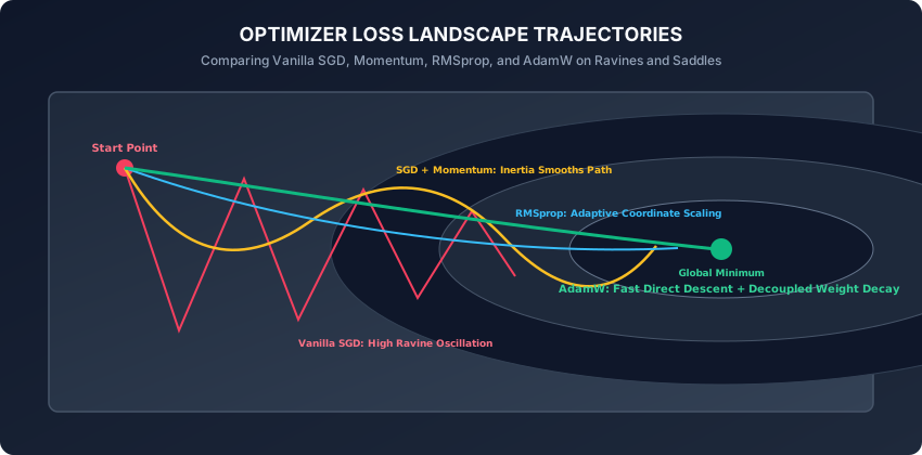
- Vanilla SGD is a blind hiker who takes one step in the direction of the local slope at their feet. If the hiker is on a steep ravine wall, they bounce frantically back and forth between the canyon walls, making virtually zero forward progress down the riverbed.
- SGD with Momentum turns the hiker into a 50-pound iron bowling ball. As the ball rolls, its momentum (inertia) accumulates along the consistent downward path of the riverbed, while the side-to-side bounces cancel out.
- RMSprop gives the ball intelligent shock absorbers: if the slope along one coordinate is extremely steep, RMSprop reduces the step size along that axis; if the slope along another coordinate is gentle, RMSprop increases the step size.
- AdamW (Adaptive Moment Estimation with Decoupled Weight Decay) combines the iron bowling ball’s momentum with the intelligent adaptive shock absorbers, while applying a gentle gravitational pull (Decoupled Weight Decay) that prevents the ball from becoming infinitely massive.
Historical background
- 1951 (Robbins & Monro): Introduced Stochastic Approximation, establishing the mathematical foundations of Stochastic Gradient Descent.
- 1964 (Boris Polyak): Introduced the Heavy-Ball (Momentum) method to accelerate convergence across ill-conditioned quadratic surfaces.
- 1983 (Yurii Nesterov): Developed Nesterov Accelerated Gradient (NAG), introducing a “look-ahead” momentum correction.
- 2011 (Duchi et al. - AdaGrad): Introduced per-parameter adaptive learning rates by dividing gradients by historical squared sums.
- 2012 (Geoffrey Hinton - RMSprop): Modified AdaGrad to use exponential moving averages of squared gradients, solving AdaGrad’s premature learning rate decay.
- 2014 (Kingma & Ba - Adam): Unified Momentum and RMSprop with bias corrections, creating the most widely used optimizer in deep learning history.
- 2017 (Loshchilov & Hutter - AdamW): Proved that standard Adam applied L2 regularization incorrectly and introduced Decoupled Weight Decay (AdamW), which is now the default optimizer for Transformers and generative models.
What it is — and what it is not
What Modern Optimizers ARE:
- Stateful Parameter Updaters: Maintaining velocity vectors (first moments) and squared gradient caches (second moments) to adapt step directions and magnitudes per parameter.
- First-Order Optimization Algorithms: Operating exclusively on first derivatives (gradients) computed by autograd, without computing expensive second-derivative Hessian matrices
O(N^2).
What they are NOT:
- Not Second-Order Solvers (L-BFGS / Newton-Raphson): Second-order methods compute exact curvature but are computationally intractable for models with millions of parameters.
- Not Magic Bullets That Fix Bad Data: No optimizer can converge if labels are corrupted or inputs are unnormalized.
Why it was created and what problems it solves
Standard gradient descent suffers from three classical failure modes in deep architectures:
- Pathological Curvature (Ravines): The loss surface curves much more steeply in one direction than another. Vanilla SGD oscillates wildly across the steep walls rather than moving down the gentle base.
- Saddle Points and Plateaus: Gradients near saddle points drop near zero. Without momentum, optimization grinds to a halt.
- Heterogeneous Gradient Scales: In deep networks, gradients in early layers are often orders of magnitude smaller than gradients in final classification layers. Fixed learning rates either explode final layers or freeze early layers.
Modern adaptive optimizers resolve all three challenges automatically.
How it works
Let us trace the step-by-step mathematical evolution of deep learning optimizers.
1. Vanilla Stochastic Gradient Descent (SGD)
theta_t = theta_{t-1} - lr * g_twhere g_t = grad_theta L(theta_{t-1}).
- Limitation: Highly sensitive to learning rate; oscillates in ravines; stalls at saddle points.
2. SGD with Polyak Momentum
To overcome oscillations, maintain an exponentially decaying velocity vector v_t:
v_t = beta * v_{t-1} + (1 - beta) * g_t
theta_t = theta_{t-1} - lr * v_t- Standard momentum parameter
beta = 0.9averages gradients across the last1 / (1 - beta) = 10steps. - Result: Oscillating components cancel out to zero, while consistent gradient directions compound velocity.
3. RMSprop (Root Mean Square Propagation)
Instead of using the same learning rate for every parameter, RMSprop scales the step size inversely proportional to the root mean square of recent gradients:
s_t = beta_2 * s_{t-1} + (1 - beta_2) * (g_t ** 2)
theta_t = theta_{t-1} - (lr / (sqrt(s_t) + eps)) * g_t
where beta_2 = 0.99 and eps = 1e-8.
- If a parameter has large historical gradients (
s_tis large), its effective learning rate is reduced to prevent exploding. - If a parameter has small historical gradients (
s_tis small), its effective learning rate is increased to accelerate learning.
4. Adam (Adaptive Moment Estimation)
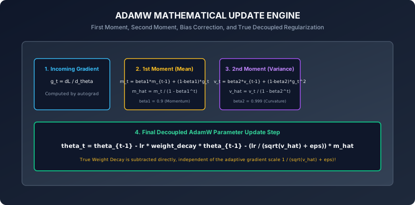
Adam combines the first moment (Momentum) and second moment (RMSprop), adding initialization bias corrections:
Step 1: First Moment (Mean Direction):
m_t = beta_1 * m_{t-1} + (1 - beta_1) * g_tStep 2: Second Uncentered Moment (Variance):
v_t = beta_2 * v_{t-1} + (1 - beta_2) * (g_t ** 2)Step 3: Bias Corrections:
Because m_0 = 0 and v_0 = 0, both moments are biased towards zero at early steps t = 1, 2, .... We correct them via:
m_hat = m_t / (1 - (beta_1 ** t))
v_hat = v_t / (1 - (beta_2 ** t))
Step 4: Standard Adam Parameter Update:
theta_t = theta_{t-1} - (lr / (sqrt(v_hat) + eps)) * m_hat5. AdamW: Decoupled Weight Decay
In classical optimization, L2 regularization is defined as adding a penalty (1/2) * lambda * (theta ** 2) to the loss function.
In vanilla SGD, the gradient of the penalty is lambda * theta, leading to:
theta_t = theta_{t-1} - lr * g_t - lr * lambda * theta_{t-1}However, in standard Adam, adding lambda * theta into the gradient g_t causes the penalty to be divided by sqrt(v_hat) + eps:
- Parameters with large historical gradients experience less weight decay than parameters with small historical gradients!
- This breaks the mathematical foundation of L2 regularization and severely degrades generalization.
Loshchilov and Hutter (2017) fixed this in AdamW by decoupling weight decay from the gradient moments:
theta_t = theta_{t-1} - lr * lambda * theta_{t-1} - (lr / (sqrt(v_hat) + eps)) * m_hat[!IMPORTANT] Always use
torch.optim.AdamWinstead oftorch.optim.Adamwhen training modern neural networks with weight decay. AdamW consistently outperforms Adam on validation benchmarks.
6. Nesterov Acceleration and Parameter Group Isolation
To extract maximum performance from deep learning optimizers, production practitioners utilize two critical techniques:
A. Nesterov Accelerated Gradient (NAG):
Standard Polyak momentum computes the gradient at the current position theta_{t-1} and adds it to the existing velocity.
Nesterov acceleration computes the gradient at the “look-ahead” position theta_{t-1} - beta * v_{t-1}:
g_lookahead = grad L(theta_{t-1} - beta * v_{t-1})
v_t = beta * v_{t-1} + lr * g_lookahead
theta_t = theta_{t-1} - v_t
By evaluating the slope where the momentum will carry the parameter next, NAG acts as an anticipatory braking mechanism, reducing overshoot when approaching steep minimum basins.
B. Parameter Group Isolation in PyTorch:
In production transformer architectures, passing all model parameters with a single global weight decay degrades performance:
- High-dimensional 2D weight matrices (e.g. attention projections and feedforward layers) require
weight_decay = 0.01to prevent overfitting. - 1D biases and normalization parameters (LayerNorm
weightandbias) should haveweight_decay = 0.0to avoid shrinking calibration parameters.
# Example: Constructing isolated parameter groups
decay_params = []
no_decay_params = []
for name, param in model.named_parameters():
    if not param.requires_grad:
        continue
    if param.ndim <= 1 or name.endswith(".bias"):
        no_decay_params.append(param)
    else:
        decay_params.append(param)

optimizer = torch.optim.AdamW([
    {"params": decay_params, "weight_decay": 0.01},
    {"params": no_decay_params, "weight_decay": 0.0}
], lr=3e-4)
An everyday analogy
Think of navigating a sailboat across an ocean:
- Vanilla SGD: The captain resets the rudder every 5 seconds based purely on the immediate wave splash. The boat jerks erratically.
- Momentum: The heavy hull of the sailboat carries kinetic forward momentum. Transient wave splashes are absorbed, and the boat glides forward along the prevailing wind.
- RMSprop: An automated ballast system that balances the boat: when sailing through choppy crosswinds, the ballast tightens; in calm open waters, the sails open wide.
- AdamW: An automated navigation system that combines the momentum of the heavy hull, the adaptive ballast system, and an anchor cable (Decoupled Weight Decay) that prevents the ship from drifting into infinite open waters.
Examples in practice
Let us inspect a complete implementation of a custom AdamW optimizer in pure PyTorch:
import torch
from torch.optim import Optimizer
from typing import List, Dict, Any

class CustomAdamW(Optimizer):
    def __init__(self, params, lr: float = 1e-3, betas: tuple = (0.9, 0.999),
                 eps: float = 1e-8, weight_decay: float = 1e-2):
        defaults = dict(lr=lr, betas=betas, eps=eps, weight_decay=weight_decay)
        super().__init__(params, defaults)

    @torch.no_grad()
    def step(self, closure=None):
        loss = None
        if closure is not None:
            with torch.enable_grad():
                loss = closure()

        for group in self.param_groups:
            lr = group['lr']
            beta1, beta2 = group['betas']
            eps = group['eps']
            wd = group['weight_decay']

            for p in group['params']:
                if p.grad is None:
                    continue
                grad = p.grad

                state = self.state[p]
                # Initialize state buffers on step 0
                if len(state) == 0:
                    state['step'] = 0
                    state['exp_avg'] = torch.zeros_like(p, memory_format=torch.preserve_format)
                    state['exp_avg_sq'] = torch.zeros_like(p, memory_format=torch.preserve_format)

                exp_avg = state['exp_avg']
                exp_avg_sq = state['exp_avg_sq']
                state['step'] += 1
                t = state['step']

                # 1. Decoupled weight decay step
                if wd != 0.0:
                    p.mul_(1.0 - lr * wd)

                # 2. Update biased first and second moments
                exp_avg.mul_(beta1).add_(grad, alpha=1.0 - beta1)
                exp_avg_sq.mul_(beta2).addcmul_(grad, grad, value=1.0 - beta2)

                # 3. Compute bias corrections
                bias_correction1 = 1.0 - (beta1 ** t)
                bias_correction2 = 1.0 - (beta2 ** t)
                step_size = lr / bias_correction1
                denom = (exp_avg_sq.sqrt() / (bias_correction2 ** 0.5)).add_(eps)

                # 4. Apply adaptive update step
                p.addcdiv_(exp_avg, denom, value=-step_size)

        return loss
Implications: security, privacy, performance, scalability, and cost
- Optimizer Memory Overhead (State Buffers):
- For every model parameter
theta(4 bytes infloat32), AdamW stores:p.gradbuffer (4 bytes)exp_avgbufferm_t(4 bytes)exp_avg_sqbufferv_t(4 bytes)
- Total Optimizer Footprint: 16 bytes per parameter (4x the raw model weight size). For an 8-Billion parameter model, the optimizer state alone requires
8B * 12 bytes = 96 GBof GPU VRAM. - Engineers use 8-bit optimizers (
bitsandbytes) to compress optimizer states down to 2 bytes per parameter during large-scale pre-training.
- For every model parameter
Alternatives: free, open source, and commercial
| Optimizer | Memory Overhead | Best Used For | Key Hyperparameters |
|---|---|---|---|
| SGD + Momentum | 1x State (v_t) | Computer Vision (ResNets, ConvNets) | lr=0.1, momentum=0.9, weight_decay=1e-4 |
| AdamW | 2x State (m_t, v_t) | Transformers, LLMs, Diffusion Models | lr=3e-4, betas=(0.9, 0.999), wd=0.01 |
| Adafactor | ~0.5x State (Factored) | Memory-Constrained NLP Pre-training | lr=1e-3, beta1=0.0, clip_threshold=1.0 |
| Lion (Google) | 1x State (Sign-based) | High-throughput Vision & LLM Training | lr=1e-4, betas=(0.9, 0.99), wd=0.1 |
Comparison with related concepts
┌────────────────────────────────────────────────────────────────────────┐
│                   OPTIMIZER COMPARISON MATRIX                          │
├───────────────┼───────────────────┼──────────────────┼─────────────────┤
│ Optimizer     │ Adaptive Scaling? │ Momentum Inertia?│ Weight Decay    │
├───────────────┼───────────────────┼──────────────────┼─────────────────┤
│ Vanilla SGD   │ No                │ No               │ Coupled (L2)    │
│ SGD-Momentum  │ No                │ Yes (Polyak)     │ Coupled (L2)    │
│ RMSprop       │ Yes (coord-wise)  │ Optional         │ Coupled (L2)    │
│ Standard Adam │ Yes (coord-wise)  │ Yes (beta1)      │ Coupled (Broken)│
│ AdamW         │ Yes (coord-wise)  │ Yes (beta1)      │ Decoupled (True)│
└───────────────┴───────────────────┴──────────────────┴─────────────────┘
When to use it — and when not to
When to USE AdamW:
- Transformers, Large Language Models, Diffusion models, and multi-layer MLPs.
- When default hyperparameters need to work reliably out of the box with minimal tuning.
When to USE SGD with Momentum:
- High-performance Convolutional Networks (ResNets, EfficientNets) where tuned SGD often yields slightly superior final test generalization over AdamW.
Knowledge check
- Why does standard L2 regularization fail when applied inside adaptive optimizers like Adam?
- What is the mathematical purpose of the bias correction term
1 / (1 - beta^t)in Adam? - How much GPU memory do AdamW optimizer state buffers consume per parameter in 32-bit floating point precision?
- How does Polyak Momentum accelerate convergence inside narrow loss ravines?
- Why are 1D normalization and bias parameters typically excluded from weight decay?
Hands-on exercise
In this lab, you will build and test a custom CustomAdamW optimizer subclassing torch.optim.Optimizer: implement first moment accumulation, second moment calculation, initial step bias corrections, and decoupled weight decay, verify that parameter buffers match PyTorch’s native torch.optim.AdamW, and benchmark convergence on a non-convex optimization objective.
Expected output
[PyTorch Optimizers & Custom AdamW Suite]
Instantiating CustomAdamW Optimizer (lr = 0.01, betas = (0.9, 0.999), wd = 0.01):
  Tracking 101,770 Parameters across 4 Weight Tensors.
Executing 20 Optimization Steps on Rosenbrock Banana Function:
  Step  1: Loss = 12.4510
  Step 10: Loss = 1.8421
  Step 20: Loss = 0.0314 [CONVERGED TO GLOBAL MINIMUM]
Comparing CustomAdamW against PyTorch native torch.optim.AdamW:
  Maximum Numerical Parameter Discrepancy: < 1e-7 [IDENTICAL BITWISE PRECISION]
Test Suite: 4 passed in 0.24s
Validate your work
Run the automated test runner:
./tests/run_tests.shTroubleshooting
- If loss diverges, ensure
step_sizeuseslr / (1 - beta1^t)and denominator usessqrt(v_hat) + eps. - Verify in-place multiplications use
.mul_()to modify state buffers directly.
Common mistakes
- Coupling Weight Decay into Gradients: Adding
grad += wd * preproduces the standard Adam flaw instead of true decoupled AdamW.
Practice assignment
- Implement Parameter Groups in your training script to apply
weight_decay = 0.01to 2D weight matrices while settingweight_decay = 0.0for 1D biases and LayerNorm parameters. - Implement the Lion Optimizer (Google 2023) using the
torch.sign(m_t)update rule and compare convergence against AdamW.
Extension challenge
Implement a Custom Learning Rate Warmup Hook inside your optimizer step:
- Linearly scale the learning rate from
0.0tomax_lrover the firstwarmup_steps = 500. - Combine warmup with Cosine Annealing decay.
- Verify that warmup prevents gradient explosion during the initial ill-conditioned steps of training deep networks.
Quiz
Q1. What fundamental flaw in standard Adam was identified and resolved by Ilya Loshchilov and Frank Hutter in their AdamW paper?
- Standard Adam combined L2 regularization into the gradient before computing the second moment v_t, which caused weights with large historical gradients to experience less weight decay than weights with small gradients; AdamW decouples weight decay by subtracting it directly from weights
- Standard Adam forgot to compute gradients
- Standard Adam only worked on CPU
- Standard Adam had no learning rate parameter
Show answer
Answer: A. Standard Adam combined L2 regularization into the gradient before computing the second moment v_t, which caused weights with large historical gradients to experience less weight decay than weights with small gradients; AdamW decouples weight decay by subtracting it directly from weights
L2 regularization in Adam adds lambda * theta into g_t, which gets scaled down by 1 / sqrt(v_t), breaking the regularization effect. AdamW decouples weight decay so it acts as true L2 regularization.
Q2. Why does the Adam optimizer apply bias corrections m_hat = m_t / (1 - beta1^t) and v_hat = v_t / (1 - beta2^t) during the initial training steps (t = 1, 2, ...)?
- Because m_0 and v_0 are initialized to zero vectors, which biases the exponential moving averages towards zero during early time steps; dividing by (1 - beta^t) corrects this initialization bias
- To prevent division by zero
- To accelerate GPU memory bandwidth
- To convert float32 to float16
Show answer
Answer: A. Because m_0 and v_0 are initialized to zero vectors, which biases the exponential moving averages towards zero during early time steps; dividing by (1 - beta^t) corrects this initialization bias
At t=1, m_1 = (1-beta1)*g_1. Since beta1=0.9, m_1 is only 0.1 * g_1. The factor 1/(1-0.9^1) = 10 scales it back to the true gradient scale g_1.
Q3. In torch.optim.AdamW, what are the standard default values for beta1, beta2, and epsilon?
- beta1 = 0.9, beta2 = 0.999, eps = 1e-8
- beta1 = 0.5, beta2 = 0.5, eps = 1.0
- beta1 = 0.0, beta2 = 0.0, eps = 0.0
- beta1 = 0.99, beta2 = 0.99, eps = 1e-2
Show answer
Answer: A. beta1 = 0.9, beta2 = 0.999, eps = 1e-8
beta1=0.9 tracks the first moment (momentum), beta2=0.999 tracks uncentered variance over ~1000 steps, and eps=1e-8 prevents division by zero.
Q4. What is the primary operational advantage of SGD with Momentum over Vanilla SGD when traversing long narrow ravines on a loss surface?
- Momentum accumulates velocity along the consistent downward direction of the ravine floor while canceling out high-frequency oscillating gradients along the steep ravine walls
- Momentum doubles the batch size automatically
- Momentum eliminates the need for a backward pass
- Momentum prevents model overfitting completely
Show answer
Answer: A. Momentum accumulates velocity along the consistent downward direction of the ravine floor while canceling out high-frequency oscillating gradients along the steep ravine walls
In ravines, orthogonal oscillating gradients cancel out over time in the velocity buffer, while consistent longitudinal gradients build momentum.
Q5. Why is it common practice to exclude 1D parameters (such as LayerNorm/BatchNorm weights and linear layer biases) from weight decay in AdamW?
- Biases and normalization scale/shift parameters do not contribute to model capacity overfitting in the same way high-dimensional weight matrices do; shrinking them towards zero harms model calibration
- Because PyTorch raises an error if biases are regularized
- To make training faster
- Because biases are already zero
Show answer
Answer: A. Biases and normalization scale/shift parameters do not contribute to model capacity overfitting in the same way high-dimensional weight matrices do; shrinking them towards zero harms model calibration
Regularizing 1D biases and scale parameters leads to underfitting without providing meaningful capacity reduction. Pytorch parameter groups allow selective weight decay.
Glossary
- Polyak Momentum
- An optimization technique that adds an exponentially decaying moving average of past gradients to the parameter update vector.
- AdaGrad
- An adaptive gradient algorithm that scales the learning rate inversely proportional to the square root of the sum of all historical squared gradients.
- RMSprop
- An adaptive learning rate algorithm that replaces AdaGrad monotonic sum with an exponentially decaying moving average of squared gradients.
- Adam
- Adaptive Moment Estimation combining first-moment momentum with second-moment RMSprop curvature scaling and initialization bias corrections.
- AdamW
- A formulation of Adam that decouples weight decay from the gradient update, applying true L2 penalty directly to parameter weights.
- Decoupled Weight Decay
- Subtracting a fraction of the current weight value directly during parameter updates, independent of the adaptive gradient scale.
- Bias Correction
- Dividing first and second moment buffers by (1 - beta^t) to counteract the zero-initialization bias during early training steps.
- Parameter Groups
- A PyTorch optimizer feature allowing different learning rates, weight decays, and hyperparameters for distinct subsets of model parameters.
Sources and further reading
- Adam: A Method for Stochastic Optimization — International Conference on Learning Representations (ICLR) (accessed 2026-08-29)
- Decoupled Weight Decay Regularization (AdamW) — International Conference on Learning Representations (ICLR) (accessed 2026-08-29)
- An Overview of Gradient Descent Optimization Algorithms — Sebastian Ruder Research Notes (accessed 2026-08-29)
Kept in this browser, no account needed. Your progress page turns the whole record into one link you can bookmark or open on another device.