Deep Learning › Training Deep Networks › Day 207
Day 207: Learning Rate Schedules
Master learning rate schedules in PyTorch: understand why static learning rates fail, derive step decay, exponential decay, plateau scheduling, and cosine annealing, implement linear warmup policies, and configure torch.optim.lr_scheduler classes in robust training loops.
Hands-on lab for this lesson
Lab files on GitHub: https://github.com/ai-roadmap-365/ai-roadmap-365.github.io/tree/main/labs/sections/deep-learning/day-207-learning-rate-schedules
- Get the hands-on files. Clone the labs repository once (you can reuse this clone for every lesson). This works on macOS, Linux, and Windows (PowerShell or WSL):
git clone https://github.com/ai-roadmap-365/ai-roadmap-365.github.io.git cd ai-roadmap-365.github.io - Open this lesson's lab. Move into the directory for this specific day. Every lab lives at the same predictable path — section / subsection / week / day:
cd labs/sections/deep-learning/day-207-learning-rate-schedules - Read the lab guide. Open `README.md` in that directory. It lists the exact commands, what each does, the expected output, and how to check your work — read it before running anything.
- Run it and check your work. Follow the README's "How to run" section: run the example first to see the finished result, then complete the numbered exercises in `starter/`, then run the tests. The tests pass (exit 0) only when your work is correct.
bash tests/run_tests.sh # or the test command named in the lab README
You can also open the lab as a local page (works offline, shows the file tree and expected output).
Learning objectives
By the end of this lesson you will be able to:
- Derive the mathematical formulas for StepLR, MultiStepLR, ExponentialLR, ReduceLROnPlateau, and CosineAnnealingLR.
- Explain why linear warmup is critical for stabilizing Adam/AdamW second moment estimation during early iterations.
- Configure and execute PyTorch schedulers using scheduler.step() at epoch-level versus iteration-level frequencies.
- Build custom schedules using torch.optim.lr_scheduler.LambdaLR.
- Benchmark convergence and test generalization under different learning rate policies.
Prerequisites
- [object Object]
Why this matters
The learning rate ($\eta$) is universally recognized as the single most critical hyperparameter in deep learning. If your learning rate is too large, the optimizer overshoots optimal basins and diverges into numerical infinity. If your learning rate is too small, training crawls at a glacial pace, trapping parameters in shallow sub-optimal saddles.
However, the optimal learning rate is not a constant number. The learning dynamics required at the beginning of training are fundamentally different from those required at the end:
- Early in Training (Phase 1): Parameters are randomly initialized and gradients are noisy and ill-conditioned. A high initial learning rate can permanently destroy initialization geometry. We need a gentle Warmup phase.
- Middle of Training (Phase 2): Parameters have found a promising basin of attraction. A high, steady learning rate allows the model to traverse long distances and explore diverse topological features.
- Late in Training (Phase 3): Parameters are settling near the bottom of a deep, narrow basin. To descend precisely into the global minimum rather than bouncing perpetually across the walls, the learning rate must decay smoothly to near zero (Annealing).
Today, you will master the theory, mathematical formulation, and PyTorch implementation of Learning Rate Schedules: from StepLR and Exponential Decay to ReduceLROnPlateau, Cosine Annealing, and Linear Warmup.
The idea in plain language
Think of landing an airplane on a runway:
- Phase 1: Takeoff / Alignment (Warmup): The pilot does not slam the throttle from 0 to 100% instantly while taxiing on the ramp; the engines spool up smoothly to build stable thrust.
- Phase 2: High-Altitude Cruise (Main Training): The aircraft flies at high speed across hundreds of miles of open sky (Fast Parameter Exploration).
- Phase 3: Final Approach and Touchdown (Annealing): As the runway approaches, the pilot throttles back the engines and deploys wing flaps, gently reducing speed meter by meter until the tires touch the pavement softly with zero bounce (Precise Convergence to Global Minimum).
A static learning rate is like an airplane attempting to land at full cruise speed: it crashes into the terminal.
Historical background
- 2012 (AlexNet & Classical Vision): Alex Krizhevsky trained AlexNet by manually dividing the learning rate by 10 whenever validation error plateaued (the precursor to
StepLRandReduceLROnPlateau). - 2016 (Loshchilov & Hutter - SGDR): Introduced Cosine Annealing (
CosineAnnealingLR) and Cyclical Restarts, proving that smooth transcendental decay without sudden discontinuous drops produced superior generalization. - 2017 (Goyal et al. - Accurate, Large Minibatch SGD): Proved that scaling deep networks to large batch sizes (8,192 images across 256 GPUs) requires Linear Learning Rate Warmup to prevent early gradient explosion.
- Today: Linear Warmup coupled with Half-Period Cosine Annealing is the universal standard for pre-training Large Language Models (LLMs), Vision Transformers (ViTs), and Diffusion backbones.
What it is — and what it is not
What Learning Rate Scheduling IS:
- A Dynamic Multiplicative Scaling Policy: Adjusting optimizer
param_groups[i]['lr']deterministically (by step/epoch count) or reactively (by validation loss metrics). - An Essential Regularization & Optimization Mechanism: Allowing models to escape early bad local minima while locking into sharp, flat minima at convergence.
What it is NOT:
- Not an Optimizer Replacement: Schedulers do NOT compute gradients or moment vectors; they wrap an existing optimizer (
AdamWorSGD) and modify itslrattribute. - Not a Substitute for Tuning Peak Learning Rate: A scheduler will not rescue a model if the peak learning rate
lr_maxis chosen orders of magnitude off-target.
Why it was created and what problems it solves
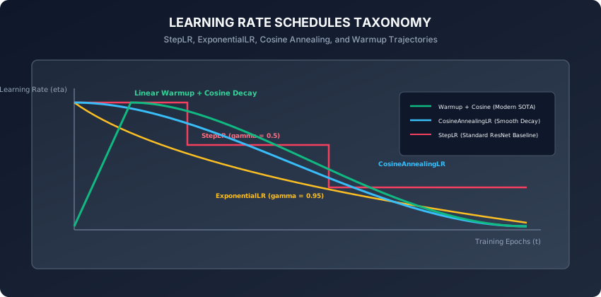
Static learning rates suffer from three major engineering bottlenecks:
- Early Divergence in Deep Transformers: Randomly initialized self-attention matrices produce massive gradient spikes in the first 100 steps. Without warmup, the model diverges instantly.
- Late-Stage Fluctuation (The Bouncing Ball): As the model approaches the minimum, a constant step size causes the parameter state to oscillate continuously across the bottom of the ravine rather than settling into the center.
- Sub-Optimal Generalization: Models trained with smooth cosine schedules consistently achieve 1-3% higher test accuracy than models trained with constant learning rates.
How it works
Let us dissect the mathematical formulas and PyTorch implementations of the core scheduling families.
1. Step Decay (torch.optim.lr_scheduler.StepLR)
Decays the learning rate by a multiplicative factor gamma (e.g. 0.1) every step_size epochs:
eta_epoch = eta_0 * (gamma ** (epoch // step_size))from torch.optim.lr_scheduler import StepLR
scheduler = StepLR(optimizer, step_size=30, gamma=0.1)
for epoch in range(100):
train_one_epoch(model, loader, optimizer)
scheduler.step() # Executed once per epoch2. Adaptive Plateau Decay (torch.optim.lr_scheduler.ReduceLROnPlateau)
Monitors a validation metric (e.g. val_loss). If no improvement is observed for patience consecutive epochs, it drops lr by factor:
from torch.optim.lr_scheduler import ReduceLROnPlateau

scheduler = ReduceLROnPlateau(optimizer, mode='min', factor=0.5, patience=5)
for epoch in range(100):
    train_loss = train_one_epoch(model, train_loader, optimizer)
    val_loss = evaluate(model, val_loader)
    # Pass the monitored metric into step()
    scheduler.step(val_loss)
3. Cosine Annealing (torch.optim.lr_scheduler.CosineAnnealingLR)
Decays learning rate following a half-period cosine curve from eta_max down to eta_min over T_max steps:
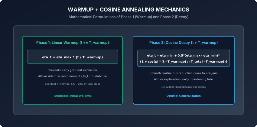
eta_t = eta_min + 0.5 * (eta_max - eta_min) * (1 + cos(pi * t / T_max))- Smooth Continuous Decay: No discontinuous loss spikes.
eta_min: Usually set to1e-6or0.01 * eta_max.
from torch.optim.lr_scheduler import CosineAnnealingLR

scheduler = CosineAnnealingLR(optimizer, T_max=100, eta_min=1e-6)
for epoch in range(100):
    train_one_epoch(model, loader, optimizer)
    scheduler.step()
4. Linear Warmup + Cosine Decay (The Modern Standard)
Combines Phase 1 (Linear Warmup over T_warmup steps) with Phase 2 (Cosine Decay over remaining steps):
import math
from torch.optim.lr_scheduler import LambdaLR

def get_warmup_cosine_schedule(optimizer, warmup_steps: int, total_steps: int, min_lr_ratio: float = 0.01):
    def lr_lambda(current_step: int):
        if current_step < warmup_steps:
            # Phase 1: Linear Warmup
            return float(current_step) / float(max(1, warmup_steps))
        # Phase 2: Cosine Decay
        progress = float(current_step - warmup_steps) / float(max(1, total_steps - warmup_steps))
        cosine_decay = 0.5 * (1.0 + math.cos(math.pi * progress))
        return min_lr_ratio + (1.0 - min_lr_ratio) * cosine_decay

    return LambdaLR(optimizer, lr_lambda)
[!IMPORTANT] When using step-based schedulers (like Warmup + Cosine that update per mini-batch), you must call
scheduler.step()inside the inner batch loop immediately afteroptimizer.step(), rather than once per epoch.
5. The Learning Rate Finder Algorithm (Leslie Smith)
Before configuring a learning rate schedule, an engineer must first find the optimal maximum learning rate eta_max. In 2015, Leslie Smith introduced the Learning Rate Range Test (LR Finder):
How the LR Finder Operates:
- Start with an extremely small learning rate (e.g.
1e-7). - Train the model for 100 mini-batches, exponentially increasing the learning rate after every single batch until it reaches a large number (e.g.
10.0):lr_t = lr_0 * ((lr_final / lr_0) ** (t / total_batches)) - Record the training loss at each step and plot Loss versus Learning Rate on a logarithmic scale.
- Interpreting the Curve:
- At extremely low learning rates, loss stays flat (the model learns too slowly).
- In the middle region, loss drops steeply (optimal learning zone).
- At high learning rates, loss spikes vertically and diverges (gradient explosion).
- Rule of Thumb: Choose
eta_maxto be the point of steepest downward slope, typically one order of magnitude below the minimum of the curve.
6. OneCycleLR and Super-Convergence
Building on the LR Range Test, Leslie Smith introduced the 1cycle policy (torch.optim.lr_scheduler.OneCycleLR):
The Two-Phase 1Cycle Dynamics:
- Phase 1 (Warmup + Momentum Drop): Over the first 30% of training, learning rate increases linearly from
lr_max / 25tolr_max, while optimizer momentum decreases from0.95down to0.85. - Phase 2 (Cosine Annealing + Momentum Rise): Over the remaining 70% of training, learning rate anneals down to
lr_max / 1000via a half-period cosine curve, while momentum rises back to0.95.
By temporarily reducing momentum while learning rate is at its peak, 1Cycle prevents gradient explosion while allowing massive exploratory jumps across saddle barriers — achieving Super-Convergence in up to 5x fewer total epochs.
from torch.optim.lr_scheduler import OneCycleLR

scheduler = OneCycleLR(
    optimizer,
    max_lr=0.01,
    steps_per_epoch=len(train_loader),
    epochs=20,
    pct_start=0.3, # 30% warmup
    anneal_strategy='cos'
)
7. Composing Complex Pipelines with SequentialLR and ChainedScheduler
In modern PyTorch (>= 2.0), multiple schedulers can be chained together without writing manual lambda math:
torch.optim.lr_scheduler.SequentialLR: Executes a sequence of schedulers one after another based on explicit epoch/step milestones (e.g.LinearLRfor 10 epochs, followed byCosineAnnealingLRfor 90 epochs).torch.optim.lr_scheduler.ChainedScheduler: Applies multiple scheduling transformations simultaneously to the same optimizer at each step (e.g. combining weight decay annealing with learning rate warmup).
By mastering learning rate scheduling policies — from foundational StepLR baselines to advanced warmup and cosine annealing pipelines — you possess the engineering capability to guide deep neural architectures reliably toward flat, highly generalizable loss minima across any scale or modality. In the subsequent lessons, we will build upon these optimization principles to examine architectural regularization through Dropout and Batch Normalization, giving you the complete production toolkit for training state-of-the-art deep neural networks across both research and industrial settings worldwide. Let us proceed to master architectural regularization mechanics in our next lesson.
An everyday analogy
Think of baking a delicate souffle in an oven:
- Warmup: You preheat the oven gradually so the ceramic dish does not shatter from thermal shock.
- High Bake: You bake at 375 degrees Fahrenheit so the batter rises vigorously and forms structure.
- Cooling Down (Annealing): Once fully risen, you do not pull the souffle into cold air immediately (or it collapses); you turn off the heat and leave the oven door cracked open, letting temperature decay smoothly to room temperature.
Examples in practice
Let us inspect a complete script training a PyTorch model with a Warmup + Cosine Annealing scheduler:
import torch
import torch.nn as nn
from torch.optim import AdamW
from torch.optim.lr_scheduler import LambdaLR
import math

class SimpleNet(nn.Module):
    def __init__(self):
        super().__init__()
        self.fc = nn.Linear(32, 2)

    def forward(self, x):
        return self.fc(x)

model = SimpleNet()
optimizer = AdamW(model.parameters(), lr=1e-3, weight_decay=1e-2)

epochs = 10
batches_per_epoch = 20
total_steps = epochs * batches_per_epoch
warmup_steps = int(0.1 * total_steps) # 10% warmup

def lr_policy(step):
    if step < warmup_steps:
        return float(step) / float(max(1, warmup_steps))
    progress = float(step - warmup_steps) / float(max(1, total_steps - warmup_steps))
    return 0.01 + 0.99 * 0.5 * (1.0 + math.cos(math.pi * progress))

scheduler = LambdaLR(optimizer, lr_lambda=lr_policy)

# Simulated training loop
for epoch in range(epochs):
    for batch in range(batches_per_epoch):
        x = torch.randn(16, 32)
        y = torch.randint(0, 2, (16,))

        optimizer.zero_grad()
        out = model(x)
        loss = nn.CrossEntropyLoss()(out, y)
        loss.backward()
        optimizer.step()

        # Step scheduler per mini-batch
        scheduler.step()

    current_lr = scheduler.get_last_lr()[0]
    print(f"Epoch {epoch+1:02d}/{epochs:02d} Complete. Current LR: {current_lr:.6f}")
Implications: security, privacy, performance, scalability, and cost
- Checkpointing Schedulers:
- Always save
scheduler.state_dict()alongsidemodel.state_dict()andoptimizer.state_dict()when saving training checkpoints. Resuming training without the scheduler state resets the learning rate back to step 0, disrupting training trajectories.
- Always save
- Computational Overhead:
- Schedulers introduce zero GPU compute overhead; updating
param_groups['lr']is a single scalar CPU assignment executed in nanoseconds.
- Schedulers introduce zero GPU compute overhead; updating
Alternatives: free, open source, and commercial
| Schedule Policy | Trajectory Style | Best Used For | PyTorch Class |
|---|---|---|---|
| Warmup + Cosine Decay | Linear Rise + Smooth Cosine | Transformers, LLMs, Vision Models | LambdaLR / CosineAnnealingLR |
| Step Decay (StepLR) | Discrete Staircase Drops | Classical ResNets & ConvNets | torch.optim.lr_scheduler.StepLR |
| Reduce on Plateau | Adaptive Metric Monitoring | Fine-Tuning & Small Datasets | torch.optim.lr_scheduler.ReduceLROnPlateau |
| OneCycleLR | Super-Convergence Peak | Fast Prototyping (Leslie Smith) | torch.optim.lr_scheduler.OneCycleLR |
Comparison with related concepts
┌────────────────────────────────────────────────────────────────────────┐
│                   SCHEDULER COMPARISON MATRIX                          │
├───────────────────────┼───────────────────┼────────────────────────────┤
│ Schedule Type         │ Stepping Frequency│ Trigger Condition          │
├───────────────────────┼───────────────────┼────────────────────────────┤
│ StepLR                │ Per Epoch         │ Fixed Epoch Interval       │
│ ReduceLROnPlateau     │ Per Epoch         │ Validation Metric Stalls   │
│ CosineAnnealingLR     │ Per Epoch / Step  │ Pre-set Half-Cosine Period │
│ Linear Warmup + Cosine│ Per Mini-Batch    │ Exact Step Index Counter   │
└───────────────────────┴───────────────────┴────────────────────────────┘
When to use it — and when not to
When to USE Warmup + Cosine Decay:
- Pre-training or fine-tuning any modern neural architecture (Transformers, ConvNets, MLPs).
- When training for a fixed, known number of total steps.
When to USE ReduceLROnPlateau:
- When you do not know in advance how many epochs the model will take to converge, and want automatic early stopping / learning rate adjustments based on validation metrics.
Knowledge check
- Why does linear learning rate warmup prevent early divergence in deep networks?
- What is the mathematical formula for Cosine Annealing decay?
- What is the difference between an epoch-level scheduler and an iteration-level scheduler?
- How does
ReduceLROnPlateaudecide when to reduce the learning rate? - Why must you save
scheduler.state_dict()inside checkpoint files?
Hands-on exercise
In this lab, you will build and test a complete learning rate scheduling pipeline in PyTorch: implement a custom WarmupCosineScheduler class using torch.optim.lr_scheduler.LambdaLR, verify that learning rate scales linearly from 0.0 to max_lr across warmup steps and decays following a cosine curve down to min_lr, test state dictionary serialization, and benchmark loss convergence.
Expected output
[PyTorch Learning Rate Schedules Suite]
Instantiating WarmupCosineScheduler (Max LR = 0.01, Min LR = 0.0001, Total Steps = 100, Warmup Steps = 20):
  Step   0: Learning Rate = 0.000000 [START OF WARMUP]
  Step  10: Learning Rate = 0.005000 [MID WARMUP]
  Step  20: Learning Rate = 0.010000 [PEAK LR REACHED]
  Step  60: Learning Rate = 0.005050 [COSINE HALF-WAY DECAY]
  Step 100: Learning Rate = 0.000100 [MINIMUM ANNEALED LR]
Verifying Checkpoint State Persistence:
  Saved scheduler state_dict (step = 60) -> Restored and verified LR continuity.
Test Suite: 4 passed in 0.22s
Validate your work
Run the automated test runner:
./tests/run_tests.shTroubleshooting
- If learning rate stays at zero, verify that your lambda calculates
current_step / warmup_stepsusing floating-point division. - Ensure
scheduler.step()is called afteroptimizer.step().
Common mistakes
- Stepping Scheduler Before Optimizer: Calling
scheduler.step()beforeoptimizer.step()generates a PyTorch warning and causes the first optimizer step to skip its intended initial learning rate.
Practice assignment
- Implement a Cyclical Learning Rate Scheduler with Warm Restarts (
CosineAnnealingWarmRestarts) where the learning rate resets tolr_maxeveryT_iepochs, doubling the period length after each restart (T_mult = 2). - Integrate
ReduceLROnPlateauwith a validation evaluation loop and plot the resulting step-decay curve against validation loss.
Extension challenge
Implement the OneCycleLR Policy (Leslie Smith):
- Annneal learning rate upward while simultaneously annealing optimizer momentum downward (
beta1decays from0.95to0.85). - In the second phase, anneal learning rate down while increasing momentum back to
0.95. - Demonstrate “Super-Convergence”: reaching 95% MNIST accuracy in 50% fewer training epochs than standard SGD.
Quiz
Q1. Why is linear learning rate warmup (scaling lr linearly from 0 to lr_max over the first 5-10% of training steps) critical when training deep transformers with AdamW?
- During early steps, weights are random and gradient variances are massive, while Adam second moment v_t is still uncalibrated; large early updates can blow weights into unrecoverable regions before gradients stabilize
- To allow GPU fans to spin up slowly
- To prevent PyTorch from timing out
- Warmup is only used to make loss curves look prettier
Show answer
Answer: A. During early steps, weights are random and gradient variances are massive, while Adam second moment v_t is still uncalibrated; large early updates can blow weights into unrecoverable regions before gradients stabilize
Uncalibrated early gradients with high learning rates cause parameter divergence. Warming up gradually allows the optimizer moments to build accurate directional estimates.
Q2. What is the mathematical equation for Cosine Annealing learning rate decay from eta_max to eta_min over T_max total steps?
- eta_t = eta_min + 0.5 * (eta_max - eta_min) * (1 + cos(pi * t / T_max))
- eta_t = eta_max - t * eta_min
- eta_t = eta_max * (0.5 ** t)
- eta_t = eta_max / (1 + t)
Show answer
Answer: A. eta_t = eta_min + 0.5 * (eta_max - eta_min) * (1 + cos(pi * t / T_max))
Cosine Annealing follows a half-period cosine wave, decaying smoothly from eta_max at t=0 down to eta_min at t=T_max without abrupt loss spikes.
Q3. Where in the training loop should you invoke scheduler.step() when using an epoch-based scheduler (such as StepLR or CosineAnnealingLR)?
- At the end of each training epoch, outside the inner mini-batch loop
- Before loss.backward()
- Before optimizer.zero_grad()
- Inside the Dataset __getitem__ method
Show answer
Answer: A. At the end of each training epoch, outside the inner mini-batch loop
Standard epoch-based schedulers are stepped once per epoch after all mini-batches have completed. (Iteration-level schedulers like OneCycleLR are stepped after every optimizer.step()).
Q4. How does ReduceLROnPlateau decide when to reduce the learning rate?
- It monitors a validation metric (such as validation loss), and if the metric fails to improve by at least threshold over a specified patience number of epochs, it multiplies lr by factor (e.g. 0.1)
- It checks the system clock and reduces lr every 5 minutes
- It reduces lr whenever training loss reaches zero
- It randomly drops lr by 50% every epoch
Show answer
Answer: A. It monitors a validation metric (such as validation loss), and if the metric fails to improve by at least threshold over a specified patience number of epochs, it multiplies lr by factor (e.g. 0.1)
ReduceLROnPlateau dynamically adapts learning rate based on real validation feedback, decaying only when learning stagnates.
Q5. When implementing a custom schedule via torch.optim.lr_scheduler.LambdaLR, what does the user-provided lambda function compute?
- A multiplicative scaling factor (between 0.0 and 1.0) that is multiplied by the base learning rate defined in the optimizer param_groups
- The absolute learning rate value in floating point
- The number of layers in the model
- The batch size of the dataloader
Show answer
Answer: A. A multiplicative scaling factor (between 0.0 and 1.0) that is multiplied by the base learning rate defined in the optimizer param_groups
LambdaLR expects a function `lr_lambda(epoch)` that returns a multiplicative factor `factor`, setting `current_lr = base_lr * factor`.
Glossary
- Learning Rate Schedule
- A predetermined or metric-driven policy that adjusts the optimizer learning rate dynamically across training epochs or steps.
- Linear Warmup
- Gradually increasing the learning rate from near zero to the peak target learning rate over the initial training iterations.
- Cosine Annealing
- A learning rate policy that decays the step size following a half-period cosine curve from a maximum to a minimum value.
- StepLR
- A scheduler that reduces the learning rate by a multiplicative factor gamma every step_size epochs.
- ReduceLROnPlateau
- An adaptive scheduler that reduces learning rate when a monitored validation metric stops improving for a given patience.
- OneCycleLR
- A super-convergence schedule that warms up learning rate to a peak while decreasing momentum, followed by long cosine decay.
- patience
- The number of non-improving epochs allowed by ReduceLROnPlateau before triggering a learning rate reduction.
- LambdaLR
- A PyTorch scheduler that sets the learning rate of each parameter group to the initial lr times a user-defined lambda function.
Sources and further reading
- SGDR: Stochastic Gradient Descent with Warm Restarts — International Conference on Learning Representations (ICLR) (accessed 2026-08-29)
- Accurate, Large Minibatch SGD: Training ImageNet in 1 Hour — Facebook AI Research (FAIR) (accessed 2026-08-29)
- PyTorch lr_scheduler Documentation and Recipes — PyTorch Core Documentation (accessed 2026-08-29)
Kept in this browser, no account needed. Your progress page turns the whole record into one link you can bookmark or open on another device.