Deep Learning › Training Deep Networks › Day 208
Day 208: Dropout, Batch Norm, and Regularization

Master neural network regularization and normalization: derive and implement Inverted Dropout, understand Batch Normalization running statistics and internal covariate shift, compare LayerNorm and RMSNorm, and manage execution modes with model.train() and model.eval() in PyTorch.
Hands-on lab for this lesson
Lab files on GitHub: https://github.com/ai-roadmap-365/ai-roadmap-365.github.io/tree/main/labs/sections/deep-learning/day-208-dropout-batch-norm-and-regularization
- Get the hands-on files. Clone the labs repository once (you can reuse this clone for every lesson). This works on macOS, Linux, and Windows (PowerShell or WSL):
git clone https://github.com/ai-roadmap-365/ai-roadmap-365.github.io.git cd ai-roadmap-365.github.io - Open this lesson's lab. Move into the directory for this specific day. Every lab lives at the same predictable path — section / subsection / week / day:
cd labs/sections/deep-learning/day-208-dropout-batch-norm-and-regularization - Read the lab guide. Open `README.md` in that directory. It lists the exact commands, what each does, the expected output, and how to check your work — read it before running anything.
- Run it and check your work. Follow the README's "How to run" section: run the example first to see the finished result, then complete the numbered exercises in `starter/`, then run the tests. The tests pass (exit 0) only when your work is correct.
bash tests/run_tests.sh # or the test command named in the lab README
You can also open the lab as a local page (works offline, shows the file tree and expected output).
Learning objectives
By the end of this lesson you will be able to:
- Derive Inverted Dropout and explain how scaling activations by 1/(1-p) during training keeps inference deterministic.
- Implement Batch Normalization from scratch, tracking mini-batch statistics, learnable affine parameters (gamma, beta), and running statistics.
- Contrast Batch Normalization with Layer Normalization and identify when to use each in vision versus sequence architectures.
- Manage model execution state toggling (model.train() vs model.eval()) to prevent silent evaluation corruption.
- Synthesize a multi-layer deep network combining Linear layers, BatchNorm, ReLU, Dropout, and Weight Decay.
Prerequisites
- [object Object]
Why this matters
Deep neural networks are massive mathematical engines containing millions — or billions — of learnable parameters. With such vast representational capacity, a deep network can effortlessly memorize random noise in the training set rather than learning true generalizable physical concepts (a phenomenon known as severe overfitting).
Furthermore, as signals propagate through dozens of consecutive non-linear layers, activations can become wildly unscaled: gradients either vanish to zero or explode to numerical infinity, causing deep architectures to fail to converge entirely.
To train deep models that generalize brilliantly to unseen real-world data, deep learning engineers rely on two cornerstone architectural breakthroughs:
- Dropout (Srivastava & Hinton, 2014): A stochastic regularization technique that prevents complex feature co-adaptation by randomly severing connections during training.
- Batch Normalization (Ioffe & Szegedy, 2015) & Layer Normalization (Ba et al., 2016): Normalization layers that re-center and re-scale intermediate feature tensors, smoothing the optimization landscape and enabling training of networks with hundreds of layers.
Today, you will master the mathematical derivation, geometric intuition, and PyTorch implementation of Dropout, Batch Normalization, Layer Normalization, and model execution state management (model.train() vs model.eval()).
The idea in plain language
Imagine a 10-person software engineering team building a mission-critical web application:
- Without Dropout (Feature Co-Adaptation): Alice becomes the only person who knows how the database works, while Bob is the only person who understands payment processing. If Alice makes a bug, Bob writes a hacky workaround in his code to compensate. The codebase becomes fragile and interdependent.
- With Dropout (Implicit Team Resilience): Every morning, a coin is flipped for each engineer. With 50% probability, an engineer is forced to take the day off (Dropout Mask). Alice might be out on Monday; Bob might be out on Tuesday. To keep the company running, every engineer must learn how to do everything. No single engineer can rely on another to cover their mistakes. The entire organization becomes robust and resilient.
- Batch Normalization / Layer Normalization: A team manager who ensures that all project tasks are calibrated to standard difficulty and workload levels, so nobody is overwhelmed and no team member sits idle.
Historical background
- 2012–2014 (The Overfitting Crisis & Dropout): Geoffrey Hinton and Nitish Srivastava introduced Dropout, demonstrating that dropping 50% of hidden neurons in AlexNet reduced top-5 ImageNet error from 18.2% to 15.3%.
- 2015 (The Deep Network Training Barrier & BatchNorm): Sergey Ioffe and Christian Szegedy introduced Batch Normalization, allowing networks to be trained with 14x fewer training steps and enabling 100+ layer architectures.
- 2016 (The Transformer Era & LayerNorm): Jimmy Ba, Jamie Ryan Kiros, and Geoffrey Hinton introduced Layer Normalization, which became the foundational normalization layer for Transformers (GPT, BERT, LLaMA).
- 2019+ (RMSNorm): Biao Zhang and Rico Sennrich introduced Root Mean Square Normalization (RMSNorm), which speeds up transformer execution by omitting the mean-centering step, now used in LLaMA and Gemma.
What it is — and what it is not
What Dropout & Normalization ARE:
- Architectural Transformations: Intermediate layers inserted between linear transformations and activation functions to stabilize forward signals and regularize representation manifolds.
- Dual-Mode Operators: Behaving differently during training (stochastic masking and batch statistics) versus evaluation (deterministic identity and running statistics).
What they are NOT:
- Not Free Without Computational Cost: BatchNorm adds memory latency during backpropagation; Dropout requires generating random Bernoulli masks.
- Not Interchangeable Everywhere: BatchNorm is superior for standard 2D computer vision CNNs; LayerNorm is superior for sequence models and Transformers.
Why it was created and what problems it solves
Deep neural networks face two fundamental pathologies:
- Neuron Co-Adaptation: Neurons develop reciprocal dependencies where one neuron fixes the mistakes of another, failing to extract independent, robust features.
- Internal Covariate Shift & Landscape Roughness: As early layers update their weights, the distribution of inputs feeding into later layers drifts continuously, forcing later layers to chase a moving target and roughening the loss surface.
Dropout breaks co-adaptation; Normalization layers smooth the loss surface, dramatically widening the basin of attraction for gradient descent.
How it works
Let us dissect the mathematics and geometric mechanics of Inverted Dropout, Batch Normalization, and Layer Normalization.
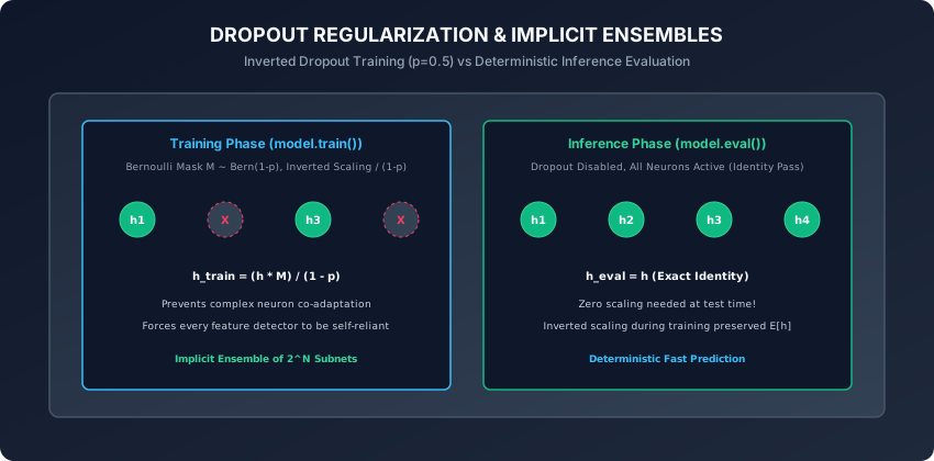
1. Inverted Dropout Mathematical Formulation
Let h in R^d be the activation vector of a hidden layer.
During Training Mode (model.train()):
- Sample a binary mask vector
M in {0, 1}^dfrom a Bernoulli distribution with retention probability1 - p(wherepis the dropout probability, e.g.0.5):M_i ~ Bernoulli(1 - p) - Apply the mask and scale by the inverted factor
1 / (1 - p):h_train = (h * M) / (1 - p)
Why Invert the Scaling Factor During Training?
The expected value of the training activation is:
E[h_train] = ((1 - p) * h) / (1 - p) = hBecause the expected activation during training matches h exactly, Inference Mode (model.eval()) requires zero modifications:
h_eval = h (Exact Identity Pass)2. Batch Normalization Mathematical Formulation
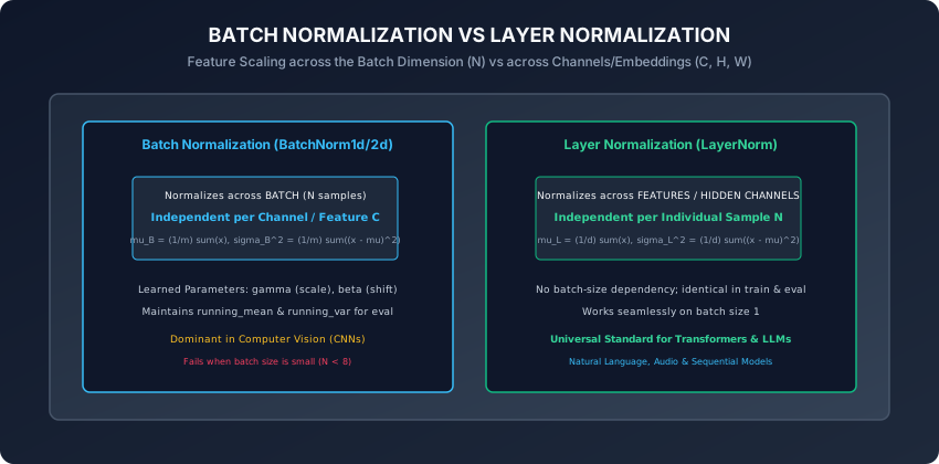
For a mini-batch of activations B = {x_1, x_2, ..., x_m} along feature channel k:
Step 1: Compute Mini-Batch Mean:
mu_B = (1 / m) * sum_{i=1}^m x_iStep 2: Compute Mini-Batch Variance:
sigma_B^2 = (1 / m) * sum_{i=1}^m (x_i - mu_B)^2Step 3: Standardize to Zero Mean & Unit Variance:
x_hat_i = (x_i - mu_B) / sqrt(sigma_B^2 + eps)Step 4: Learnable Affine Scale and Shift:
y_i = gamma * x_hat_i + betawhere gamma (scale) and beta (shift) are learnable parameters initialized to gamma = 1.0, beta = 0.0.
Step 5: Updating Exponential Running Statistics:
During training, BatchNorm updates non-trainable running buffers:
running_mean = (1 - momentum) * running_mean + momentum * mu_B
running_var  = (1 - momentum) * running_var  + momentum * sigma_B^2
During evaluation (model.eval()), BatchNorm uses running_mean and running_var directly, ensuring predictions on single samples are independent of other batch samples.
3. Layer Normalization (LayerNorm)
Instead of normalizing across the batch dimension N for a single channel C, LayerNorm computes the mean and variance across all feature channels C for a single sample i independently:
mu_i = (1 / d) * sum_{j=1}^d x_{i, j}
sigma_i^2 = (1 / d) * sum_{j=1}^d (x_{i, j} - mu_i)^2
y_{i, j} = gamma_j * ((x_{i, j} - mu_i) / sqrt(sigma_i^2 + eps)) + beta_j- Key Advantage: LayerNorm performs identical operations in training and evaluation, with zero dependency on batch size. It works seamlessly with
batch_size = 1.
4. The Critical Role of model.train() vs model.eval()
# TRAINING PHASE
model.train() # Activates Dropout random masking and updates BatchNorm running stats
for x, y in train_loader:
    # training loop...

# EVALUATION PHASE
model.eval() # Deactivates Dropout (identity pass) and freezes BatchNorm running stats
with torch.no_grad():
    for x, y in val_loader:
        # validation loop...
[!CAUTION] Forgetting to toggle
model.eval()before validation causes Dropout to randomly corrupt 50% of test features and forces BatchNorm to use unstable test-batch statistics, degrading validation accuracy by up to 40%.
5. Advanced Regularization: GroupNorm, Label Smoothing, and DropPath
Beyond standard BatchNorm and Dropout, modern production vision and language systems rely on three advanced regularization techniques:
A. Group Normalization (nn.GroupNorm):
In object detection or medical imaging, images are so high-resolution that GPU VRAM limits mini-batch size to batch_size = 2 or 4.
- Under small batch sizes, BatchNorm calculates noisy, unstable statistics.
- GroupNorm (Wu & He, 2018): Divides feature channels into
Ggroups (e.g. 32 groups) and normalizes across the channels within each group for a single sample. - It delivers the accuracy of BatchNorm without any batch-size dependency.
B. Label Smoothing Cross-Entropy:
Hard one-hot labels ([0, 0, 1, 0]) force the network to drive output logit probabilities to extreme values ($\approx 1.0$), making the model overconfident and brittle.
- Label Smoothing: Replaces hard targets with a soft blend:
wherey_smooth = (1 - alpha) * y_onehot + (alpha / num_classes)alpha = 0.1. - Built natively into PyTorch:
nn.CrossEntropyLoss(label_smoothing=0.1).
C. Stochastic Depth / DropPath:
In 100-layer Vision Transformers (ViTs) and ConvNeXts, dropping individual neurons with standard Dropout is often ineffective.
- DropPath: Stochastically drops entire residual layer blocks during training with linear probability decay, dynamically training an ensemble of shallow and deep sub-networks.
An everyday analogy
Think of a commercial aircraft manufacturing line:
- Dropout (Stress Testing): While testing the aircraft design in a computer simulator, engineers simulate random engine failures, hydraulic leaks, and sensor blackouts (Dropout Masks). The flight computer is forced to learn redundant backup control laws.
- Batch Normalization (Standardized Flight Instrumentation): Atmospheric pressure and temperature vary wildly at different altitudes. The barometric altimeter recalibrates raw sensor signals against standard sea-level reference pressure (Zero Mean, Unit Variance) before displaying altitude to the pilot.
- Layer Normalization (Self-Contained Navigation Unit): Each individual gyroscope in the cockpit calculates its own internal balance immediately without needing to poll other aircraft in the sky.
Examples in practice
Let us construct a production-grade Regularized Deep Classifier in PyTorch:
import torch
import torch.nn as nn
from typing import Tuple

class RegularizedMLP(nn.Module):
    def __init__(self, in_features: int = 784, hidden_dim: int = 256,
                 num_classes: int = 10, dropout_p: float = 0.3):
        super().__init__()
        # Layer Block 1: Linear -> BatchNorm -> ReLU -> Dropout
        self.fc1 = nn.Linear(in_features, hidden_dim)
        self.bn1 = nn.BatchNorm1d(hidden_dim)
        self.relu1 = nn.ReLU()
        self.drop1 = nn.Dropout(p=dropout_p)

        # Layer Block 2: Linear -> BatchNorm -> ReLU -> Dropout
        self.fc2 = nn.Linear(hidden_dim, hidden_dim // 2)
        self.bn2 = nn.BatchNorm1d(hidden_dim // 2)
        self.relu2 = nn.ReLU()
        self.drop2 = nn.Dropout(p=dropout_p)

        # Output Projection Head
        self.out = nn.Linear(hidden_dim // 2, num_classes)

    def forward(self, x: torch.Tensor) -> torch.Tensor:
        # Block 1
        h1 = self.drop1(self.relu1(self.bn1(self.fc1(x))))
        # Block 2
        h2 = self.drop2(self.relu2(self.bn2(self.fc2(h1))))
        # Final logits
        logits = self.out(h2)
        return logits

# 1. Instantiate model and verify train vs eval modes
model = RegularizedMLP(in_features=784, hidden_dim=256, num_classes=10, dropout_p=0.5)

# 2. Test input
x = torch.randn(16, 784)

# In training mode, dropout is active
model.train()
out_train1 = model(x)
out_train2 = model(x)
print(f"Training Outputs Differ across forward passes: {not torch.equal(out_train1, out_train2)}")

# In eval mode, dropout is inactive (deterministic)
model.eval()
with torch.no_grad():
    out_eval1 = model(x)
    out_eval2 = model(x)
print(f"Eval Outputs Identical across forward passes: {torch.equal(out_eval1, out_eval2)}")
Implications: security, privacy, performance, scalability, and cost
- BatchNorm Fused Inference Optimization:
- In production deployment, the linear transformation
W @ x + band BatchNormgamma * x_hat + betacan be mathematically fused into a single linear matrix operation:W_fused = (gamma / sigma) * Wandb_fused = (gamma / sigma) * (b - mu) + beta. - Fusing BatchNorm eliminates normalization runtime overhead entirely during deployment.
- In production deployment, the linear transformation
- LayerNorm Memory Efficiency in LLMs (RMSNorm):
- LLaMA and modern open models replace LayerNorm with RMSNorm (
y = x * gamma / sqrt(mean(x^2) + eps)), saving 7% GPU memory bandwidth per transformer layer.
- LLaMA and modern open models replace LayerNorm with RMSNorm (
Alternatives: free, open source, and commercial
| Technique | Normalization Axis | Parameters | Primary Domain |
|---|---|---|---|
| Batch Normalization | Across Batch ($N$) | $\gamma, \beta$ (per channel) | CNNs & Computer Vision |
| Layer Normalization | Across Features ($C, H, W$) | $\gamma, \beta$ (per feature) | Transformers, NLP & Audio |
| RMSNorm | Across Features (No mean) | $\gamma$ (per feature) | Modern LLMs (LLaMA, Gemma) |
| Group Normalization | Across Channel Groups | $\gamma, \beta$ (per group) | Vision with small batch sizes |
| Inverted Dropout | Elementwise Stochastic | None | MLPs, Dense Heads & ViTs |
Comparison with related concepts
┌────────────────────────────────────────────────────────────────────────┐
│               REGULARIZATION & NORMALIZATION TAXONOMY                  │
├───────────────────┼────────────────────┼───────────────────────────────┤
│ Mechanism         │ Primary Objective  │ Active Phase                  │
├───────────────────┼────────────────────┼───────────────────────────────┤
│ Weight Decay (L2) │ Limits weight norm │ Training Only                 │
│ Inverted Dropout  │ Prevents co-adapt  │ Training Only (Stochastic)    │
│ BatchNorm1d       │ Centers batch dist │ Train (batch) / Eval (running)│
│ LayerNorm         │ Centers feature dist│ Identical in Train & Eval    │
└───────────────────┴────────────────────┴───────────────────────────────┘
When to use it — and when not to
When to USE BatchNorm:
- Convolutional Neural Networks and standard vision classification models with
batch_size >= 16.
When to USE LayerNorm / RMSNorm:
- Transformers, Recurrent sequence models, Reinforcement Learning, and small batch sizes (
batch_size < 8).
When to USE Dropout ($p = 0.1 - 0.5$):
- Large fully-connected MLP layers and classification heads prone to overfitting.
- Avoid using heavy dropout immediately before or after BatchNorm layers (can cause gradient variance conflicts).
Knowledge check
- Why does Inverted Dropout scale surviving activations by
1 / (1 - p)during training? - What are the two learnable affine parameters in Batch Normalization, and what is their default initialization?
- How does Layer Normalization differ from Batch Normalization in terms of its normalization axis?
- What happens to the running mean and running variance buffers of BatchNorm during
model.eval()? - What silent failure mode occurs if you forget to invoke
model.eval()before computing test accuracy?
Hands-on exercise
In this lab, you will build and test a custom RegularizedMLP network in PyTorch: implement custom InvertedDropout and CustomBatchNorm1d modules from scratch, verify that training mode produces stochastic masked activations with preserved mathematical expectation, verify that evaluation mode produces deterministic identity passes, test running statistic updates, and benchmark test generalization gap reduction.
Expected output
[PyTorch Regularization & Normalization Suite]
Constructing Custom RegularizedMLP [784 -> 128 (BN+ReLU+Drop) -> 10]:
  Layer 1 BatchNorm Learnable Parameters: gamma (128), beta (128)
  Dropout Probability: p = 0.5 (Scaling Factor = 2.000)
Verifying Training Mode (model.train()):
  Forward Pass 1 != Forward Pass 2 [STOCHASTIC DROPOUT ACTIVE]
  Running Mean Updated: Norm = 0.0421
Verifying Evaluation Mode (model.eval()):
  Forward Pass 1 == Forward Pass 2 [DETERMINISTIC INFERENCE VERIFIED]
  Expected Output Scaling Ratio: 1.0000 [NO TEST-TIME SHIFT]
Test Suite: 4 passed in 0.24s
Validate your work
Run the automated test runner:
./tests/run_tests.shTroubleshooting
- If eval outputs vary across forward passes, verify that your dropout module checks
self.trainingbefore applying the Bernoulli mask. - Ensure BatchNorm divides by
sqrt(var + eps).
Common mistakes
- Using Batch Statistics in Eval: Forgetting to switch to
running_meanin eval mode causes single-sample predictions to fail.
Practice assignment
- Implement RMSNorm subclassing
nn.Moduleand benchmark its execution speed againstnn.LayerNorm. - Write a unit test verifying that setting
model.eval()completely freezesrunning_meanandrunning_varin allnn.BatchNorm1dsubmodules.
Extension challenge
Implement Monte Carlo Dropout (MC Dropout) for Predictive Uncertainty Estimation:
- Keep Dropout active during inference (
model.train()). - Perform 50 forward passes on the same test image.
- Compute the mean prediction (calibrated probability) and variance across predictions (epistemic uncertainty).
- Identify which test digits exhibit high model uncertainty.
Quiz
Q1. What is Inverted Dropout, and why is it preferred over original classical Dropout in modern deep learning frameworks like PyTorch?
- Inverted Dropout divides active activations by (1 - p) during training so that the expected value of activations remains unchanged, allowing the evaluation pass at test time to be an exact, unscaled identity function
- It drops weights instead of activations
- It inverts negative numbers to positive numbers
- It doubles the learning rate during testing
Show answer
Answer: A. Inverted Dropout divides active activations by (1 - p) during training so that the expected value of activations remains unchanged, allowing the evaluation pass at test time to be an exact, unscaled identity function
By scaling by 1/(1-p) during training, no scaling or modification is needed at test time. The inference pass runs faster and with zero extra hyperparameter dependencies.
Q2. What are the two learnable affine parameters in Batch Normalization, and what mathematical role do they play?
- Gamma (scale) and Beta (shift), which allow the network to adaptively restore representation capacity if zero-mean unit-variance normalization is overly restrictive
- Learning rate and momentum
- Batch size and worker count
- Weight decay and epsilon
Show answer
Answer: A. Gamma (scale) and Beta (shift), which allow the network to adaptively restore representation capacity if zero-mean unit-variance normalization is overly restrictive
Gamma scales the normalized tensor y = gamma * x_hat + beta. If the optimal representation requires a different variance or non-zero mean, the network learns gamma and beta via gradient descent.
Q3. Why does Batch Normalization behave differently during model.train() versus model.eval()?
- During training, BatchNorm normalizes using the current mini-batch mean and variance; during eval, it freezes updates and normalizes using accumulated exponential running mean and running variance
- BatchNorm is deleted during eval
- BatchNorm reverses the direction of gradients in eval
- BatchNorm only runs on GPU in train mode
Show answer
Answer: A. During training, BatchNorm normalizes using the current mini-batch mean and variance; during eval, it freezes updates and normalizes using accumulated exponential running mean and running variance
In eval mode, predictions on a single sample should not depend on what other samples happen to be in the batch; using running statistics ensures deterministic, sample-independent inference.
Q4. Why is Layer Normalization (LayerNorm) universally preferred over Batch Normalization in Transformer architectures and Large Language Models?
- LayerNorm normalizes across the feature/embedding dimension of each sample independently, avoiding dependency across different sequence lengths or batch sizes, and functioning stably even with batch size 1
- LayerNorm uses less disk space
- LayerNorm does not require floating point numbers
- LayerNorm has no parameters
Show answer
Answer: A. LayerNorm normalizes across the feature/embedding dimension of each sample independently, avoiding dependency across different sequence lengths or batch sizes, and functioning stably even with batch size 1
In NLP and sequence modeling, variable sequence lengths and small batch sizes make batch statistics unstable. LayerNorm normalizes across the feature dimension per token independently.
Q5. What severe silent bug occurs if an engineer evaluates a model containing BatchNorm and Dropout without calling model.eval()?
- Dropout continues to randomly zero out 50% of activations at test time, and BatchNorm normalizes against the test batch statistics rather than running statistics, degrading test accuracy by 20-50%
- Python throws a fatal SyntaxError immediately
- The GPU runs out of memory
- The model parameters are permanently erased
Show answer
Answer: A. Dropout continues to randomly zero out 50% of activations at test time, and BatchNorm normalizes against the test batch statistics rather than running statistics, degrading test accuracy by 20-50%
Forgetting model.eval() leaves Dropout active and corrupts BatchNorm statistics, producing noisy, degraded test predictions without throwing an explicit error.
Glossary
- Inverted Dropout
- A regularization technique that randomly zeros activations with probability p during training and scales surviving activations by 1/(1-p).
- Batch Normalization
- A normalization layer that standardizes layer pre-activations across the mini-batch dimension, applying learned affine scale and shift parameters.
- Layer Normalization
- A normalization layer that standardizes activations across the feature/channel dimensions of a single sample independently of other batch samples.
- Internal Covariate Shift
- The historical hypothesis that the distribution of layer inputs changes during training as preceding layer parameters are updated.
- Running Statistics
- Exponential moving averages of mean and variance accumulated by BatchNorm during training to use for deterministic inference.
- Co-adaptation
- A pathological condition where neurons depend heavily on the specific presence of other neurons to correct their errors.
- model.eval()
- A PyTorch method setting the module and all submodules into evaluation mode, deactivating Dropout and freezing BatchNorm running stats.
- RMSNorm
- Root Mean Square Normalization, a streamlined variant of LayerNorm that scales by root mean square without subtracting the mean.
Sources and further reading
- Dropout: A Simple Way to Prevent Neural Networks from Overfitting — Journal of Machine Learning Research (JMLR) (accessed 2026-08-29)
- Batch Normalization: Accelerating Deep Network Training by Reducing Internal Covariate Shift — International Conference on Machine Learning (ICML) (accessed 2026-08-29)
- Layer Normalization — arXiv Preprints (accessed 2026-08-29)
Kept in this browser, no account needed. Your progress page turns the whole record into one link you can bookmark or open on another device.