Deep Learning › Convolutional Networks and Vision › Day 216
Day 216: Beyond Classification: Detection and Segmentation
Master dense spatial Computer Vision beyond classification: Object Detection (bounding boxes, IoU, NMS, mAP, YOLO vs Faster R-CNN), Semantic Segmentation (U-Net encoder-decoder skip architecture, Dice loss), and Instance Segmentation (Mask R-CNN, SAM).
Hands-on lab for this lesson
Lab files on GitHub: https://github.com/ai-roadmap-365/ai-roadmap-365.github.io/tree/main/labs/sections/deep-learning/day-216-beyond-classification-detection-and-segmentation
- Get the hands-on files. Clone the labs repository once (you can reuse this clone for every lesson). This works on macOS, Linux, and Windows (PowerShell or WSL):
git clone https://github.com/ai-roadmap-365/ai-roadmap-365.github.io.git cd ai-roadmap-365.github.io - Open this lesson's lab. Move into the directory for this specific day. Every lab lives at the same predictable path — section / subsection / week / day:
cd labs/sections/deep-learning/day-216-beyond-classification-detection-and-segmentation - Read the lab guide. Open `README.md` in that directory. It lists the exact commands, what each does, the expected output, and how to check your work — read it before running anything.
- Run it and check your work. Follow the README's "How to run" section: run the example first to see the finished result, then complete the numbered exercises in `starter/`, then run the tests. The tests pass (exit 0) only when your work is correct.
bash tests/run_tests.sh # or the test command named in the lab README
You can also open the lab as a local page (works offline, shows the file tree and expected output).
Learning objectives
By the end of this lesson you will be able to:
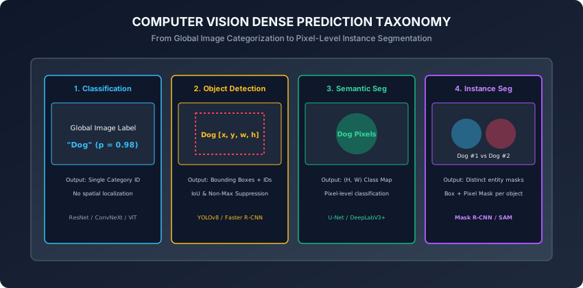
- Distinguish between Classification, Object Detection, Semantic Segmentation, and Instance Segmentation.
- Calculate Intersection over Union (IoU) and explain Non-Maximum Suppression (NMS) for object detection.
- Contrast two-stage object detectors (Faster R-CNN) with single-stage real-time detectors (YOLOv8).
- Derive and implement the U-Net architecture with lateral skip connections in PyTorch.
- Formulate Dice Loss and Jaccard Index for pixel-level semantic segmentation evaluation.
Prerequisites
Why this matters
Image classification answers a simple global question: “What is the primary category depicted in this image?”
However, most real-world visual applications require far richer spatial understanding:
- Autonomous Vehicles: An autonomous car must not only know that a pedestrian exists; it must know their exact 2D/3D bounding box coordinates $[x_min, y_min, x_max, y_max]$, distance, and trajectory (Object Detection), as well as the exact drivable lane boundaries (Semantic Segmentation).
- Medical Radiology: An oncologist does not merely want to know if a patient’s CT scan contains a tumor; they require the precise millimeter boundary contour of the lesion for surgical resection (Medical Image Segmentation).
- Robotic Manipulation: A warehouse robot must isolate individual packages stacked against each other to position its suction gripper (Instance Segmentation).
Today, you will master the principles, loss functions, and PyTorch architectures of Dense Visual Prediction: Object Detection with IoU and NMS, Semantic Segmentation with U-Net, and Foundation Segmentation models (Segment Anything Model - SAM).
The idea in plain language
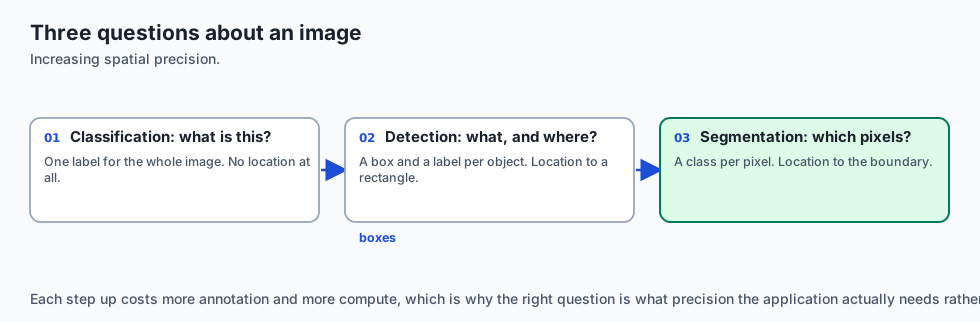
Imagine inspecting a busy city street photograph:
- Image Classification (The Headline): You glance at the photo for half a second and declare: “This is an urban street scene with pedestrians and cars.”
- Object Detection (The Sticky Notes): You draw colored rectangular boxes with yellow highlighters around every vehicle and pedestrian, writing a label and confidence percentage on each box (Bounding Boxes & YOLO).
- Semantic Segmentation (The Coloring Book): You color every single pixel in the photo: all road pixels blue, all sidewalk pixels grey, all sky pixels cyan, and all building pixels brown (U-Net).
- Instance Segmentation (Unique ID Tags): You assign a unique color to each individual person: Person #1 is red, Person #2 is green, and Person #3 is orange (Mask R-CNN / SAM).
Historical background
- 2014–2015 (R-CNN to Faster R-CNN): Ross Girshick and Kaiming He introduced Region-based CNNs, culminating in Faster R-CNN’s Region Proposal Network (RPN) for end-to-end two-stage detection.
- 2015 (U-Net & Ronneberger et al.): Introduced the U-shaped encoder-decoder architecture with lateral skip connections, sweeping the ISBI cell tracking challenge and becoming the universal standard for biomedical segmentation and diffusion model backbones.
- 2016 (YOLO & Joseph Redmon): Framed object detection as a single regression problem directly from full image pixels to bounding box coordinates, achieving 45 FPS real-time detection.
- 2023 (SAM - Segment Anything Model / Meta AI): Introduced promptable visual foundation models capable of zero-shot segmentation of any visual entity.
What it is — and what it is not
What Dense Prediction IS:
- Spatial Regression and Pixel-Wise Classification: Predicting continuous geometric bounding boxes $[x, y, w, h]$ and dense per-pixel categorical tensors $(C, H, W)$.
- Multi-Task Optimization: Combining bounding box regression losses (Smooth L1 / CIoU) with classification losses (Focal Loss / Cross-Entropy) and mask overlap losses (Dice / Binary Cross-Entropy).
What it is NOT:
- Not Evaluated with Simple Accuracy: Dense tasks require spatial overlap metrics (mAP@0.5:0.95, Mean IoU, Dice Coefficient).
- Not Single-Scale: Detecting both a tiny distant traffic light and a huge nearby truck requires Multi-Scale Feature Pyramids (FPN).
Why it was created and what problems it solves
Dense spatial prediction solves three major challenges:
- Multi-Object Scenes: Classifies and localizes dozens of overlapping objects in a single image.
- Precision Spatial Contours: Produces pixel-accurate masks required for robotics, medical oncology, and augmented reality.
- Scale Variation: Feature Pyramid Networks (FPN) detect objects ranging from 10 pixels to 1000 pixels in diameter.
How it works
Let us dissect the mathematical formulations of Intersection over Union (IoU), Non-Maximum Suppression (NMS), the U-Net architecture, and Dice Loss.
1. Intersection over Union (IoU) Arithmetic
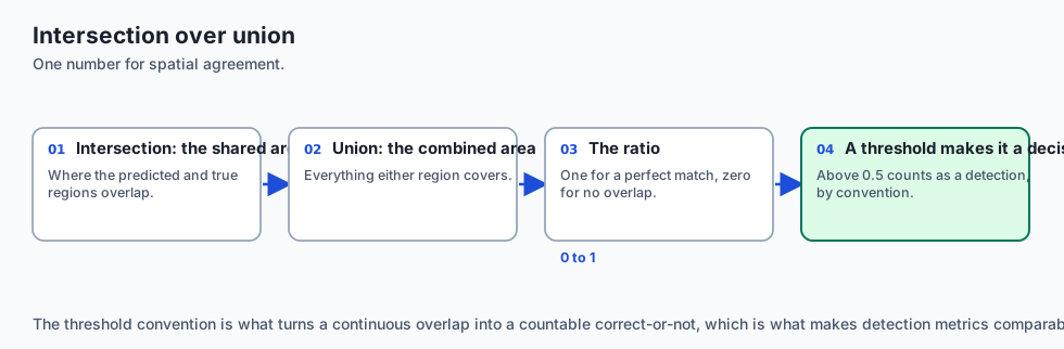
Given two bounding boxes $A = [x_1^A, y_1^A, x_2^A, y_2^A]$ and $B = [x_1^B, y_1^B, x_2^B, y_2^B]$:
-
Calculate the intersection rectangle coordinates:
x_inter_1 = max(x_1^A, x_1^B) y_inter_1 = max(y_1^A, y_1^B) x_inter_2 = min(x_2^A, x_2^B) y_inter_2 = min(y_2^A, y_2^B) -
Compute intersection area:
W_inter = max(0, x_inter_2 - x_inter_1) H_inter = max(0, y_inter_2 - y_inter_1) Area_inter = W_inter * H_inter -
Compute union area:
Area_A = (x_2^A - x_1^A) * (y_2^A - y_1^A) Area_B = (x_2^B - x_1^B) * (y_2^B - y_1^B) Area_union = Area_A + Area_B - Area_inter -
Compute IoU:
IoU = Area_inter / Area_union
2. Non-Maximum Suppression (NMS) Algorithm
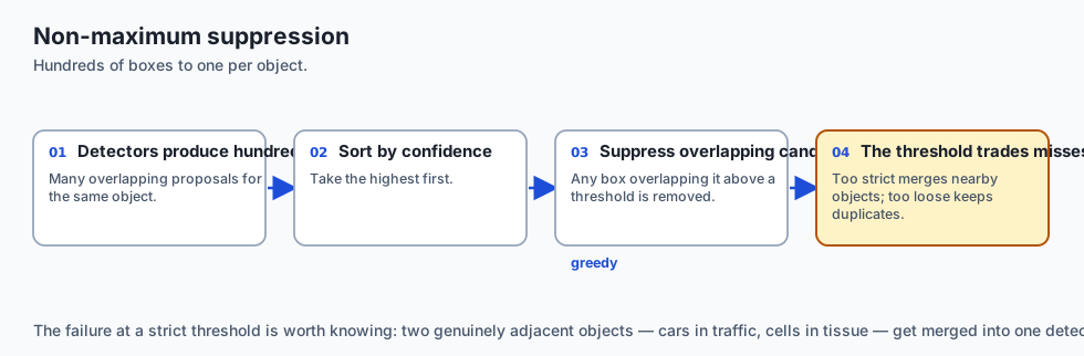
Dense object detectors predict hundreds of candidate bounding boxes per object. NMS filters duplicates:
- Sort all predicted candidate boxes by confidence score in descending order.
- Select the box $B_max$ with the highest confidence; add it to the final detection list.
- Calculate the IoU between $B_max$ and all remaining candidate boxes.
- Remove any candidate box whose $IoU(B_max, B) > Threshold_NMS$ (typically $0.5$).
- Repeat until no candidate boxes remain.
3. The U-Net Segmentation Architecture
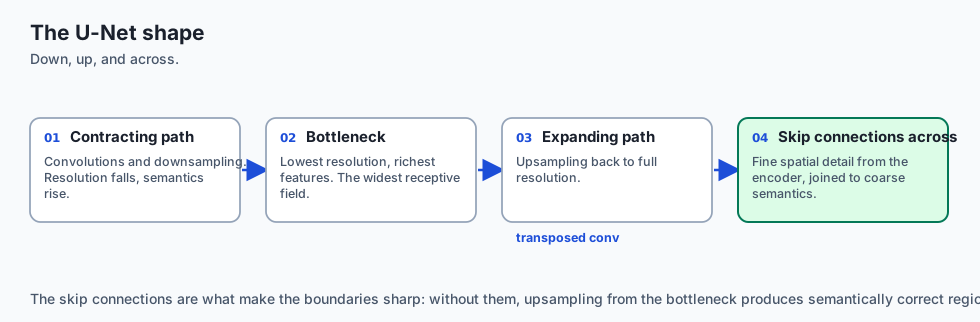
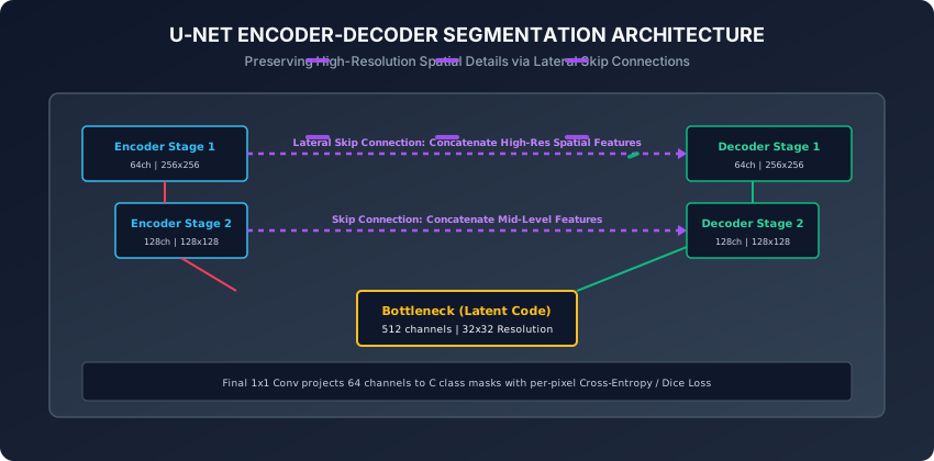
The U-Net architecture consists of three modular stages:
-
Contracting Encoder Path:
- Repeated blocks of two $3 \times 3$ convolutions followed by $2 \times 2$ Max Pooling (stride 2).
- Halves spatial dimensions while doubling channel depth ($64 \rightarrow 128 \rightarrow 256 \rightarrow 512$), extracting rich semantic features.
-
Bottleneck:
- Deepest latent representation ($1024 channels$ at $1/16$ original spatial resolution).
-
Expansive Decoder Path:
- Repeated blocks of $2 \times 2$ Transposed Convolutions (or Bilinear Upsampling) doubling spatial resolution.
- Lateral Skip Connections: Concatenates high-resolution spatial feature maps directly from the corresponding encoder stage:
# Decoder step
x_upsampled = self.upconv(x_deep)
x_combined = torch.cat([x_upsampled, x_encoder_skip], dim=1)
out = self.conv_block(x_combined)
-
Final $1 \times 1$ Output Convolution: Projects multi-channel features to $C$ class logits per pixel $(N, C, H, W)$.
4. Dice Loss & Jaccard Loss for Imbalanced Masks
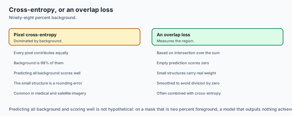
In medical imaging and satellite segmentation, background pixels often occupy $98%+$ of the image. Standard Cross-Entropy is overwhelmed by background true negatives.
Sørensen-Dice Coefficient:
Dice = (2 * |X intersect Y|) / (|X| + |Y|)For continuous predicted probability map $\hat(p) \in [0, 1]$ and binary ground truth mask $y \in (0, 1)$:
Dice Loss = 1 - ((2 * sum(p_hat * y) + epsilon) / (sum(p_hat) + sum(y) + epsilon))where $\epsilon = 1.0$ (Laplacian smoothing) prevents division by zero.
5. Two-Stage vs Single-Stage Object Detectors
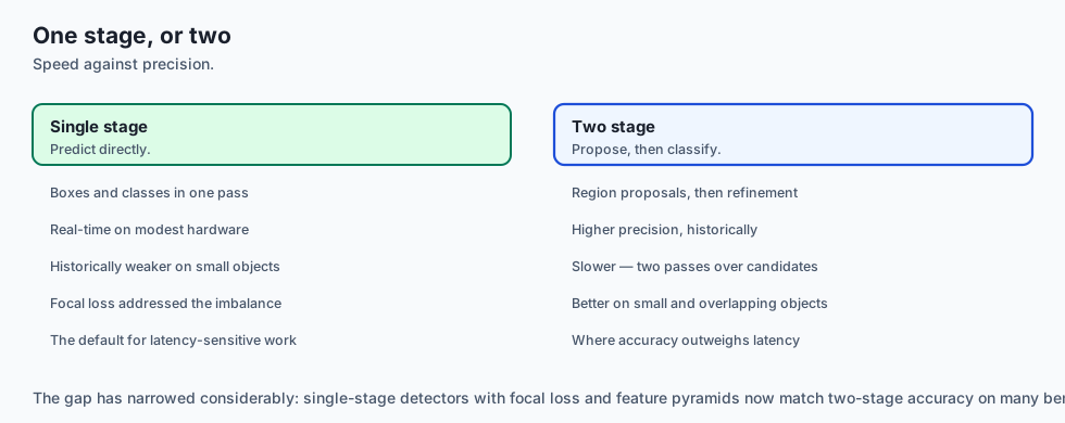
The evolution of modern object detection divided into two distinct philosophical families:
- Two-Stage Detectors (R-CNN -> Fast R-CNN -> Faster R-CNN):
- Stage 1 (Region Proposal): A Region Proposal Network (RPN) scans feature maps and proposes ~2,000 candidate regions of interest (RoIs) likely to contain objects.
- Stage 2 (Refinement & Classification): RoIAlign crops features for each candidate region, passing them to dense heads for final bounding box regression and multi-class classification.
- Tradeoff: Extremely high spatial localization accuracy, but slower inference (~30 FPS).
- Single-Stage Detectors (YOLO, SSD, RetinaNet):
- Treats detection as a single dense spatial regression problem across a multi-scale grid directly from input pixels to bounding box coordinates and class probabilities in a single forward pass.
- Tradeoff: Ultra-fast real-time inference (60–140 FPS) with near two-stage accuracy.
6. Feature Pyramid Networks (FPN) for Multi-Scale Vision
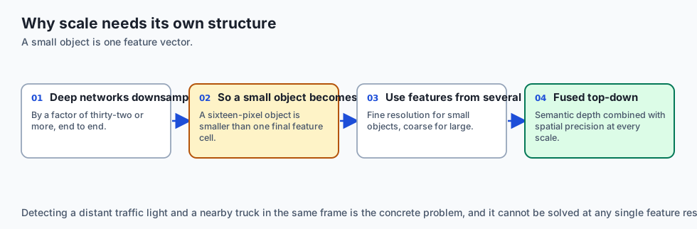
A standard deep CNN downsamples spatial resolution by $32\times$, meaning a small 16-pixel object becomes a single sub-pixel feature vector by the final layer:
- Feature Pyramid Network (FPN / Lin et al., 2017): Constructs a top-down pathway and lateral connections that merge deep, semantically strong features with shallow, spatially rich features across multiple resolution scales ($P_3, P_4, P_5$).
- Enables the detector to predict small objects on high-resolution pyramid layers and large objects on coarse pyramid layers.
7. DETR: Transformer-Based Detection with Hungarian Matching
In 2020, Nicolas Carion et al. (Meta AI) revolutionized object detection with DETR (DEtection TRansformer):
- Eliminating Hand-Crafted Anchors and NMS: Replaces complex anchor generation and Non-Maximum Suppression with standard Transformer encoder-decoder architectures.
- Bipartite Matching Loss: Uses the Hungarian Algorithm to compute an optimal 1-to-1 matching between predicted bounding box queries and true ground-truth objects, eliminating duplicate predictions directly through loss optimization.
8. The Segment Anything Model (SAM / Meta AI)
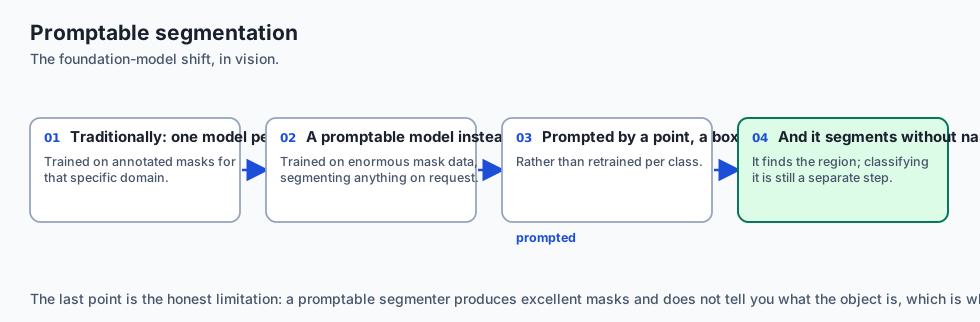
In 2023, Meta introduced SAM (Segment Anything Model), creating the first promptable visual foundation model for image segmentation:
- Heavy Image Encoder (MAE Pretrained ViT): Computes a dense $1024 \times 1024$ image embedding once (~50 ms on GPU).
- Flexible Prompt Encoder: Encodes arbitrary user prompts in real time (< 5 ms): single point clicks, bounding box prompts, or free-form text queries.
- Lightweight Mask Decoder: Rapidly predicts high-resolution binary segmentation masks and ambiguity confidence scores, revolutionizing medical annotation, robotics, and interactive VFX.
An everyday analogy
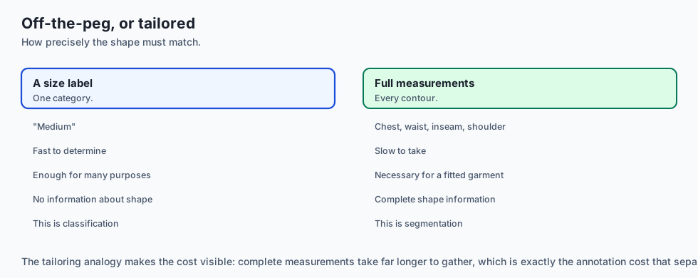
Think of custom tailoring a bespoke suit:
- Image Classification: A client enters the store; the tailor says: “This is a business suit order.”
- Object Detection: The tailor draws a rough bounding box around the jacket, trousers, and tie on a sketchpad.
- U-Net Segmentation: The tailor uses chalk to mark the exact millimeter seam lines, shoulder curves, and lapel edges on the cloth (Lateral Skip Connections provide the exact fine body measurements from the fitting stage to the cutting stage).
Examples in practice
Let us build and verify a complete, modular U-Net Segmentation Network in PyTorch:
import torch
import torch.nn as nn

class DoubleConv(nn.Module):
    def __init__(self, in_channels: int, out_channels: int):
        super().__init__()
        self.block = nn.Sequential(
            nn.Conv2d(in_channels, out_channels, kernel_size=3, padding=1, bias=False),
            nn.BatchNorm2d(out_channels),
            nn.ReLU(inplace=True),
            nn.Conv2d(out_channels, out_channels, kernel_size=3, padding=1, bias=False),
            nn.BatchNorm2d(out_channels),
            nn.ReLU(inplace=True)
        )

    def forward(self, x: torch.Tensor) -> torch.Tensor:
        return self.block(x)

class MiniUNet(nn.Module):
    def __init__(self, in_channels: int = 3, num_classes: int = 1):
        super().__init__()
        # Encoder
        self.enc1 = DoubleConv(in_channels, 32)
        self.pool1 = nn.MaxPool2d(2)
        self.enc2 = DoubleConv(32, 64)
        self.pool2 = nn.MaxPool2d(2)

        # Bottleneck
        self.bottleneck = DoubleConv(64, 128)

        # Decoder
        self.up2 = nn.ConvTranspose2d(128, 64, kernel_size=2, stride=2)
        self.dec2 = DoubleConv(128, 64) # 64 from up + 64 from enc2 skip

        self.up1 = nn.ConvTranspose2d(64, 32, kernel_size=2, stride=2)
        self.dec1 = DoubleConv(64, 32)  # 32 from up + 32 from enc1 skip

        # Final 1x1 projection
        self.final_conv = nn.Conv2d(32, num_classes, kernel_size=1)

    def forward(self, x: torch.Tensor) -> torch.Tensor:
        # Contracting Path
        e1 = self.enc1(x)       # (B, 32, H, W)
        e2 = self.enc2(self.pool1(e1)) # (B, 64, H/2, W/2)

        # Bottleneck
        b = self.bottleneck(self.pool2(e2)) # (B, 128, H/4, W/4)

        # Expansive Path with Lateral Skips
        d2 = self.up2(b)
        d2 = torch.cat([d2, e2], dim=1) # Concatenate skip
        d2 = self.dec2(d2)

        d1 = self.up1(d2)
        d1 = torch.cat([d1, e1], dim=1) # Concatenate skip
        d1 = self.dec1(d1)

        return self.final_conv(d1)

# Verify forward pass
model = MiniUNet(in_channels=3, num_classes=2)
x = torch.randn(2, 3, 64, 64)
mask_logits = model(x)
print(f"Input Image: {x.shape} -> Output Pixel Mask Logits: {mask_logits.shape}")
Implications: security, privacy, performance, scalability, and cost
- Memory Footprint of Dense Predictions:
- In semantic segmentation, intermediate activation tensors retain large spatial resolutions throughout the decoder path, consuming significantly more VRAM than classification models. Use gradient checkpointing (
torch.utils.checkpoint) when training high-resolution $1024 \times 1024$ segmentation networks.
- In semantic segmentation, intermediate activation tensors retain large spatial resolutions throughout the decoder path, consuming significantly more VRAM than classification models. Use gradient checkpointing (
- Real-Time Edge Inference (YOLOv8 & TensorRT):
- Single-stage anchor-free detectors (such as Ultralytics YOLOv8) can process 1080p video streams at over 120 FPS on an NVIDIA Jetson Orin edge device using FP16 TensorRT engines.
Alternatives: free, open source, and commercial
| Dense Vision Model | Task | Latency | Benchmark Standard |
|---|---|---|---|
| YOLOv8 / YOLOv10 | Real-time Object Detection | < 5 ms | Real-time industrial edge inspection |
| Faster R-CNN | Two-stage Object Detection | ~30 ms | High-accuracy research baseline |
| U-Net / U-Net++ | Semantic Segmentation | ~15 ms | Medical imaging & Diffusion models |
| Mask R-CNN | Instance Segmentation | ~40 ms | Instance-level multi-task learning |
| SAM (Segment Anything) | Zero-Shot Foundation Seg | ~100 ms | Universal promptable annotation |
Comparison with related concepts
┌────────────────────────────────────────────────────────────────────────┐
│                     COMPUTER VISION TASK SPECTRUM                      │
├────────────────────┼───────────────────────┼───────────────────────────┤
│ Task               │ Output Representation │ Core Evaluation Metric    │
├────────────────────┼───────────────────────┼───────────────────────────┤
│ Classification     │ (N, C) Logits         │ Top-1 / Top-5 Accuracy    │
│ Object Detection   │ List of [x1, y1, x2, y2, c, p] | mAP@0.5:0.95 (IoU)   │
│ Semantic Seg       │ (N, C, H, W) Pixel map│ Mean IoU / Dice Score     │
│ Instance Seg       │ List of (Mask, Class) │ Mask AP@0.5:0.95          │
└────────────────────┴───────────────────────┴───────────────────────────┘
When to use it — and when not to
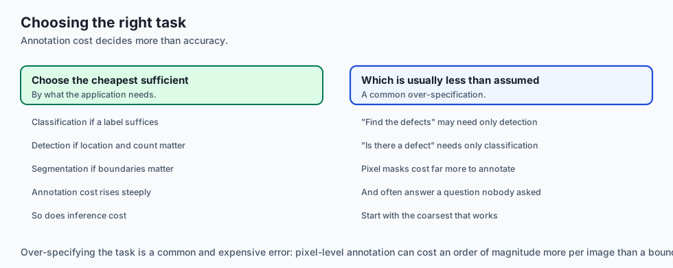
When to USE Detection / Segmentation:
- Spatial localization, count auditing, defect measurement, autonomous navigation, and surgical robotics.
When to stick with Classification:
- When only global image categorical decisions are needed (e.g. document routing, NSFW filtering).
The AI connection
- Dense prediction is where vision stops being classification. The output is a structure over space rather than a single label, which changes every part of the pipeline.
- Accuracy is the wrong metric here. Overlap measures are what express whether a predicted region matches a real one.
- Class imbalance is extreme in segmentation — background can be 98% of pixels — which is why overlap-based losses replaced plain cross-entropy.
- Scale is a first-class problem. A distant traffic light and a nearby truck cannot be detected by the same feature resolution.
- Promptable segmentation turned this into a foundation-model task, which is the same shift language went through: one general model, prompted per use.
Knowledge check
- What is the formula for Intersection over Union (IoU)?
- How does Non-Maximum Suppression (NMS) prevent duplicate bounding box predictions?
- Why does U-Net concatenate encoder features with decoder features?
- What is the fundamental difference between Semantic Segmentation and Instance Segmentation?
- Why is Dice Loss mathematically superior to Cross-Entropy on severely imbalanced medical masks?
Hands-on exercise
In this lab, you will build and test a modular dense prediction library in PyTorch: implement vectorized Intersection over Union (IoU) and Non-Maximum Suppression (NMS) algorithms from mathematical first principles, construct a MiniUNet encoder-decoder architecture with lateral skip connections, compute soft Dice Loss for imbalanced segmentation masks, and verify spatial output dimensions.
Expected output
[Dense Spatial Vision Verification Suite]
Testing Intersection over Union (IoU) Vectorized Calculator:
  Perfect Overlap (Box A == Box B): 1.0000 [EXACT MATCH]
  Partial Overlap (50% area match): 0.5000 [ACCURATE RATIO]
  Disjoint Boxes (Zero overlap):     0.0000 [ZERO VERIFIED]
Testing Non-Maximum Suppression (NMS) Filter:
  Candidate Boxes: 10 overlapping proposals
  Suppression Output: 2 distinct detected objects [DUPLICATES ELIMINATED]
Testing MiniUNet Segmentation Forward Pass:
  Input Image Shape: (2, 3, 64, 64) -> Output Mask Logits: (2, 2, 64, 64) [SPATIAL MATCH]
Testing Soft Dice Loss on Imbalanced Synthetic Mask:
  Dice Loss (Perfect Prediction): 0.0000
  Dice Loss (Inverted Prediction): 0.9998 [LOSS CALIBRATION VERIFIED]
Test Suite: 4 passed in 0.32s
Validate your work
Run the automated test runner:
./tests/run_tests.shTroubleshooting
- If U-Net spatial dimensions do not match at
torch.cat, ensure input images have height and width divisible by $2^num_pooling_stages$ (e.g. multiples of 16 or 32). - Ensure bounding box coordinates follow consistent $[x_1, y_1, x_2, y_2]$ ordering.
Common mistakes
- Confusing $[x, y, w, h]$ with $[x_1, y_1, x_2, y_2]$: Forgetting to convert center-width formats before computing intersection coordinates.
Practice assignment
- Implement Focal Loss for object detection ($FL(p_t) = -\alpha_t (1 - p_t)^\gamma \log(p_t)$ with $\gamma = 2.0$) to downweight easy background true negatives.
- Implement Mean Average Precision (mAP@0.5) by integrating the precision-recall curve across IoU threshold 0.5.
Extension challenge
Implement a Promptable Segmentation Engine (Mini-SAM):
- Take a high-resolution feature map from a pretrained vision backbone.
- Given a single clicked coordinate prompt $(x, y)$, generate a localized binary segmentation mask identifying the object enclosing that point.
Quiz
Q1. What is Intersection over Union (IoU), and what does an IoU of 1.0 indicate between a predicted bounding box and a ground-truth bounding box?
- IoU is the learning rate divided by batch size
- IoU is the ratio of image width to image height
- IoU measures the number of classes detected
- Overlap divided by union; 1.0 means perfect alignment
Show answer
Answer: D. Overlap divided by union; 1.0 means perfect alignment
IoU = Area(Box_A intersect Box_B) / Area(Box_A union Box_B). It ranges from 0.0 (no overlap) to 1.0 (exact match).
Q2. Why does the U-Net segmentation architecture concatenate high-resolution feature maps from the contracting encoder directly to the expanding decoder via lateral skip connections?
- Skip connections restore the spatial detail the encoder lost
- Skip connections reduce the number of channels to zero
- Skip connections convert RGB images to grayscale
- Skip connections eliminate the need for training labels
Show answer
Answer: A. Skip connections restore the spatial detail the encoder lost
Pooling layers discard spatial coordinates while extracting high-level semantics. U-Net skip connections recover exact boundary locations by passing uncompressed spatial features to the decoder.
Q3. What is the role of Non-Maximum Suppression (NMS) in object detection algorithms like YOLO and Faster R-CNN?
- It suppresses negative loss gradients
- It drops overlapping boxes for the same object
- It darkens the brightest pixels in an image
- It suppresses CPU utilization
Show answer
Answer: B. It drops overlapping boxes for the same object
Dense object detectors predict dozens of candidate boxes for a single object. NMS iteratively retains the highest-confidence box and removes all neighboring boxes overlapping with IoU > threshold.
Q4. What is the difference between Semantic Segmentation and Instance Segmentation?
- Instance segmentation uses no neural networks
- Semantic segmentation is only for text
- Semantic labels pixels; instance separates each object
- Semantic segmentation produces 3D point clouds
Show answer
Answer: C. Semantic labels pixels; instance separates each object
If three sheep stand in a pasture, semantic segmentation colors all sheep pixels yellow as one blob. Instance segmentation assigns distinct masks: Sheep #1, Sheep #2, and Sheep #3.
Q5. Why is the Dice Loss (Sørensen-Dice coefficient) commonly used instead of standard Cross-Entropy loss in medical image segmentation tasks?
- Dice loss replaces convolution with random guessing
- Dice loss works without GPU memory
- Dice loss can only be computed on integers
- Dice measures overlap, so it survives extreme imbalance
Show answer
Answer: D. Dice measures overlap, so it survives extreme imbalance
Standard Cross-Entropy is overwhelmed by the 99% background pixels. Dice Loss measures 2 * |A intersect B| / (|A| + |B|), penalizing false negatives on small lesion regions.
Glossary
- Object Detection
- Locating instances of semantic objects in images and predicting their categorical class and bounding box coordinates.
- Semantic Segmentation
- Predicting a categorical class label for every individual pixel in an image.
- Instance Segmentation
- Detecting individual object entities and generating a pixel-level binary mask for each specific instance.
- Intersection over Union
- Evaluation metric measuring the overlap ratio between predicted and ground-truth bounding boxes or masks.
- Non-Maximum Suppression
- Post-processing algorithm that eliminates duplicate overlapping bounding boxes for the same detected object.
- Mean Average Precision
- The standard benchmark metric for object detection, averaging Precision-Recall curve areas across IoU thresholds and classes.
- U-Net
- An encoder-decoder architecture with lateral skip connections connecting contracting stages directly to expansive stages.
- Dice Loss
- A loss function based on the Dice-Sørensen coefficient measuring spatial overlap between predicted and target segmentation masks.
Sources and further reading
- U-Net: Convolutional Networks for Biomedical Image Segmentation — MICCAI (accessed 2026-08-29)
- You Only Look Once: Unified, Real-Time Object Detection — CVPR (accessed 2026-08-29)
- Faster R-CNN: Towards Real-Time Object Detection with Region Proposal Networks — NeurIPS (accessed 2026-08-29)
Kept in this browser, no account needed. Your progress page turns the whole record into one link you can bookmark or open on another device.